The final goal of this project is to perform 3D physics simulation on objects on 2D image plane. This project is inspired by a paper presented in SIGGRAPH 2014, “3D Object Manipulation in a Single Photograph using Stock 3D Models”. In this paper, authors present a method that enables users to perform 3D manipulations to an object in a photograph assuming that the user provides a stock 3D model with components for all parts of the objects visible in the original photograph [1]. They also provide a real-time geometry correction interface for user, in order to align the 3D model to the photograph, semi-automatically.
3D manipulations often reveal some part of the object that is not visible in the photograph, in the above mentioned article, hidden parts of the object is completed according to the provided 3D model and symmetries of the object itself. As a final touch, they estimate the 3D illumination of the scene to cast realistic shadows and light effects. You can see the results and detailed information about their project here.
As for my project, I tried to implement the essence of the mentioned article and a simplified version of each task in addition to a physics simulation on the 3D model in the photograph. In this project I assume the object that we are going to manipulate is a simple box which is selected by its corners by user. I partitioned the implementation of this project into several steps shown in the following list:
Each of these steps are described and discussed in the following sections.
Paying attention to some simple conditions in selecting the input photograph might improve the results of the algorithm significantly. First of all it’s important that 3 faces of the target object are entirely visible in the image; this way, the algorithm could generate an acceptable texture map for the object. For example in the photograph below you can barely see 2 faces of the cardboard box. Therefore it would be impossible for the algorithm to generate a proper texture map for the box.
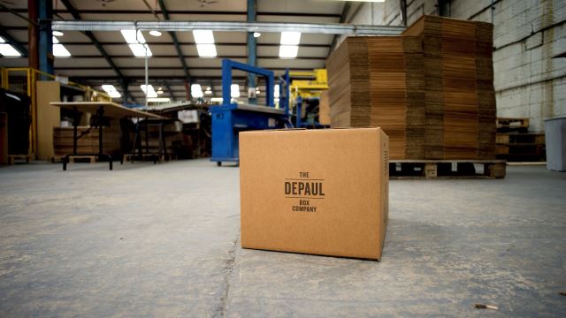
Figure 1 - A photograph in which only one face (barely 2 faces) of a cardboard box is shown
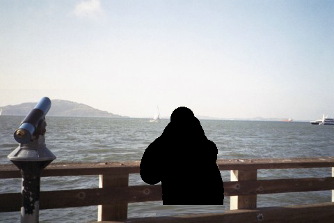
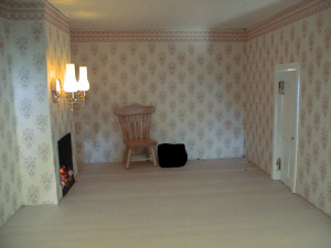
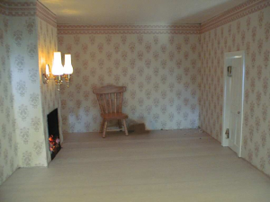
As the second tip, we should pay attention to the background of the object. For instance, as can be seen in the following photo, the object (red ottoman) has a very complicated background that could not be completely filled by the algorithm, although a good part of the carpet is filled with correct curves and colors. On the other hand, since the object is covering a part of another object (black ottoman) when we erase our object, the covered object could not be reconstruct correctly by texture synthesis. (Click to see hte images with better resolution)
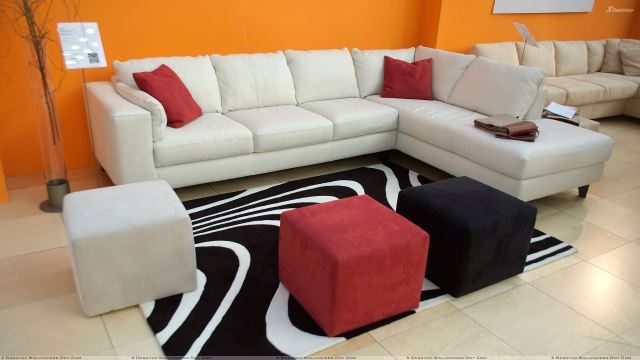
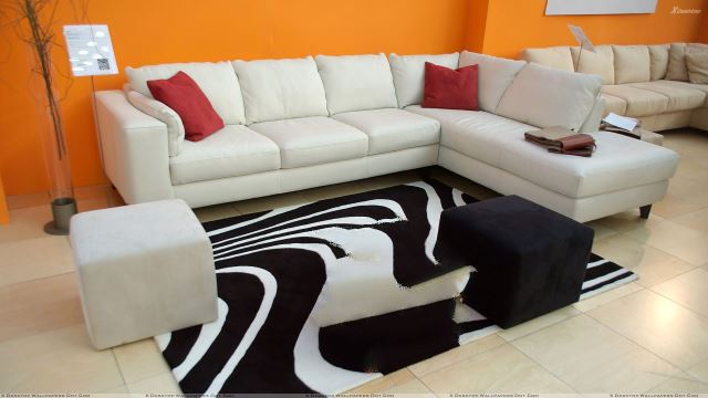
Figure 2 - Object with complicated background texture which is not filled completely
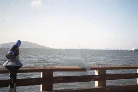
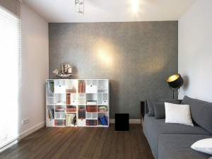
An example of an acceptable photo is shown in the following figure in which, the object (the bucket) covers nothing but continuous textures that as can be seen caused the object to be easily removed from the photograph. This is the photo that I’m going to test my algorithm on. (Click to see images with higher resolution)


Figure 3 - An example of an acceptable photo
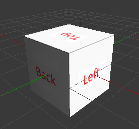
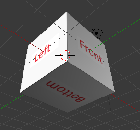
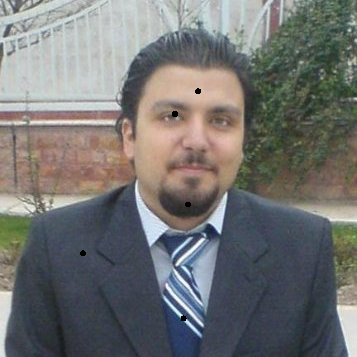
At this part, user has to select the corners of the target box and the algorithm generates a cube texture map that could be later used in Blender. I assume that in the selected photo three faces of the box is visible and by default I assume that front and top face are visible, therefore I ask user to select which side face of the box is visible (Left or Right). After that user has to select box vertices in the given order which is shown in the following figure.
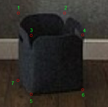
Figure 4 - User selects object's vertices in a given order
Before taking about generating a texture map, I have to talk about UV maps a little bit. UV mapping is the 3D modeling process of making a 2D image representation of a 3D model's surface. UV maps permit polygons that make up a 3D object to be painted with color from an image. The image is called a UV texture map but it's just an ordinary image [2]. In other words, UV map is an unwrapped version of the object’s surface on a 2D plain. (See the following picture)
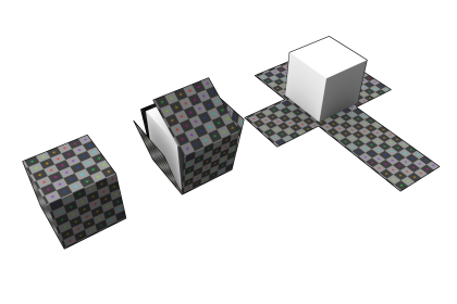
Figure 5 - UV mapping (Texture map)
Therefore if we want to paint the texture of an object we have to generate a 2D UV map for it. For this purpose we have to export an unwrapped UV map of our cube in Blender, then change this map and then reapply it to the cube.
To export an unwrapped version of our cube’s UV map we follow these steps in Blender:
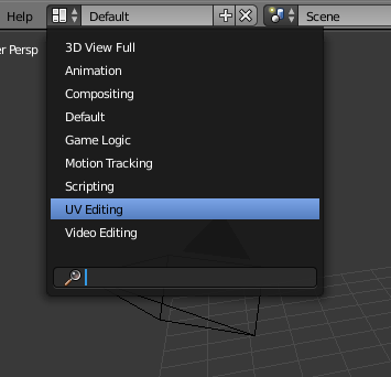
Select “UV Editing” mode from dropdown list on top of the window.
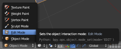
Enter “Edit mode” using the list on the bottom of the screen.
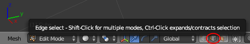
Select “Edge select” mode in the adjacent list on the bottom of the screen.
Select a snake shape sequence of the edges around the cube. (7 edges shown in the following image)
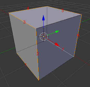
Press “Mark seam” in “Shading/UVs” tab in the middle of the screen.
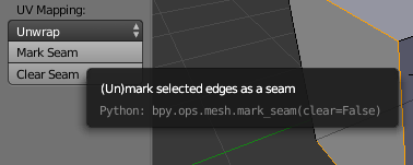
Press “A” to select all faces of the cube, press “U” and then select Unwrap.
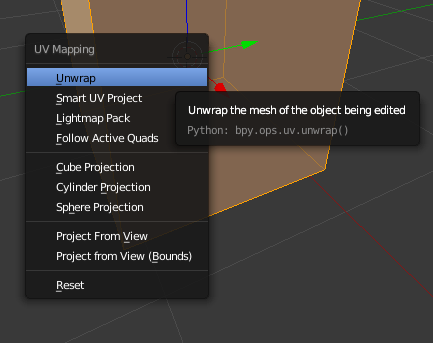
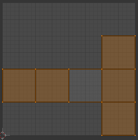
The unwrapped shape (shown in the right part of the screen) should be something like the following image.
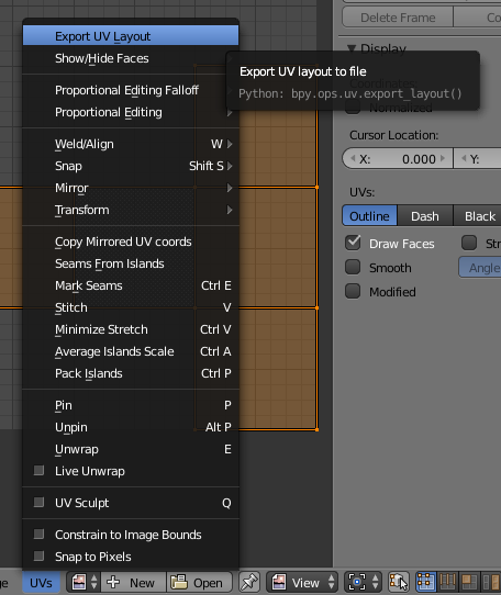
Select “Export UV Layout” from “UVs” menu on the bottom of the screen and save the UV map as an PNG image.
At the end we will have a PNG containing UV map template of our cube. Please note that this part was done only once to generate a UV map template and it doesn’t involve the user. After I obtained this template, I configured my GenerateCubeMap function in Matlab to generate UV maps according to this template. I will discuss this function further down.
As can be seen in the following image, the mentioned template is a 1024x1024 pixel image in which each face of the cube is represented by a 256x256 rectangular with a 256x1024 empty space at the top of the image. (Click for a higher resolution image)
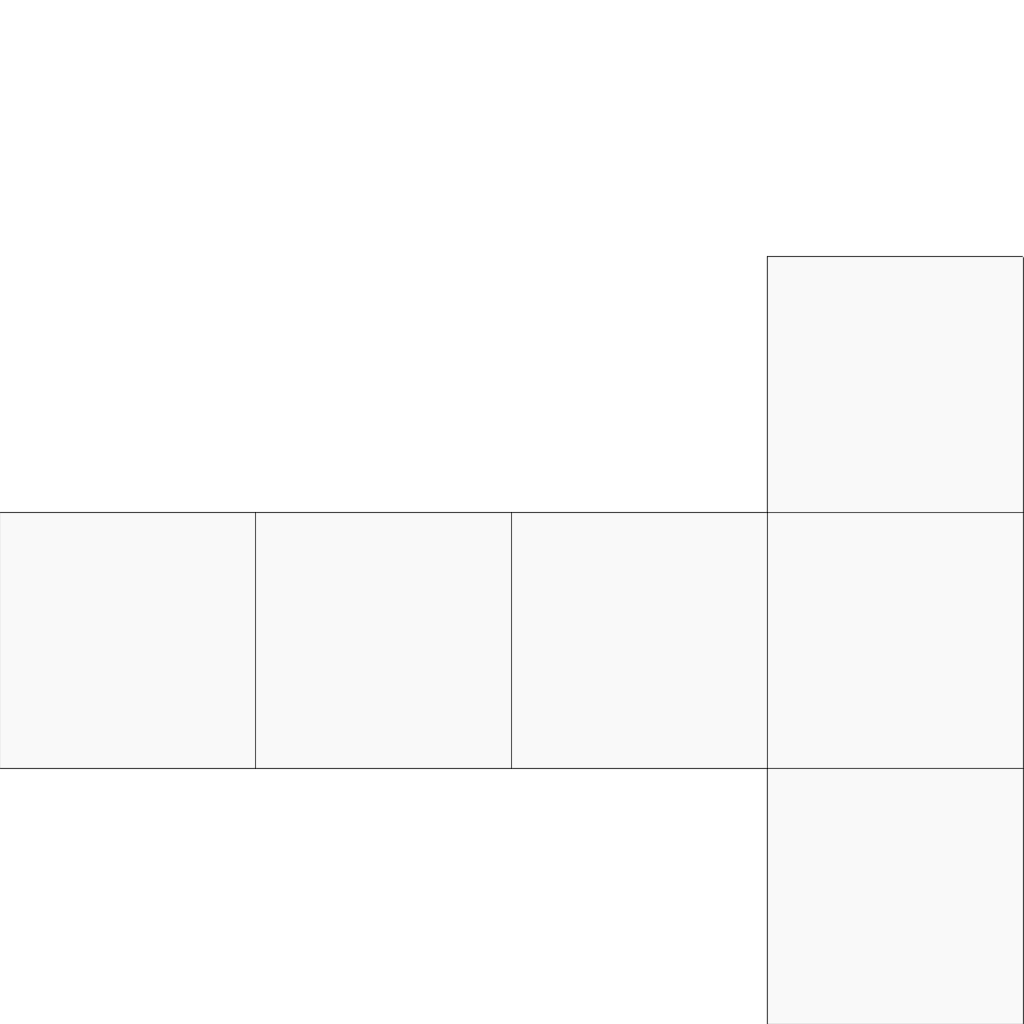
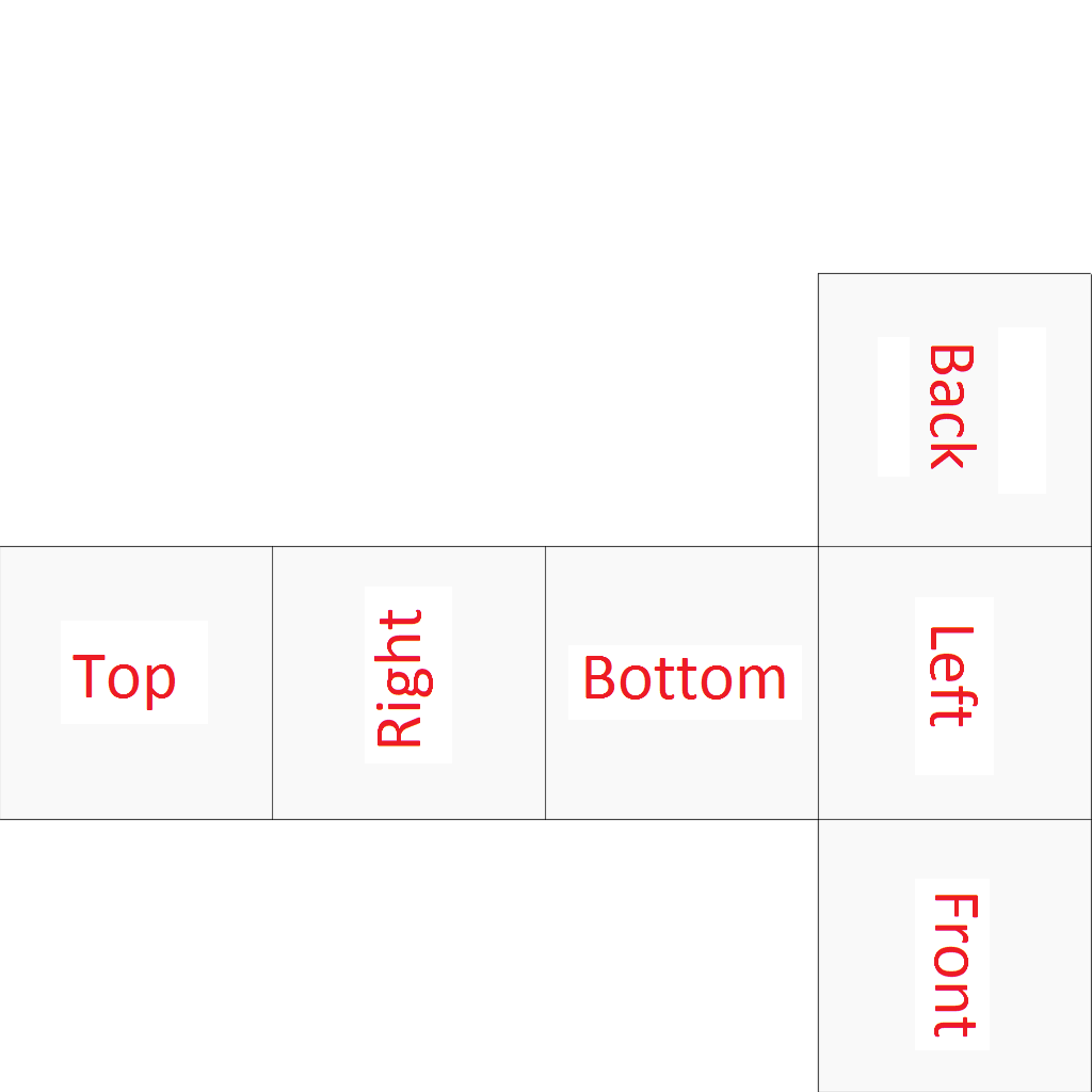
Figure 6 – (left) UV map template, (right) Placement and orientation of the faces
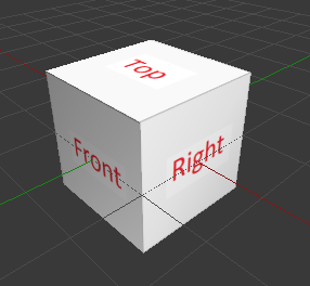
For example if I choose the image shown above (right side) as texture map for our cube, the result would be something like this:
This function calculates a homographic matrix (H) for each face of our object, using the vertices selected by user in the second step; then warps the texture of each face on its correct place in the texture map. For more information about calculating the H matrix see “Homography Estimation” in here.
For example you can see the generated texture map of the bucket shown in Figure 4 in the following image.
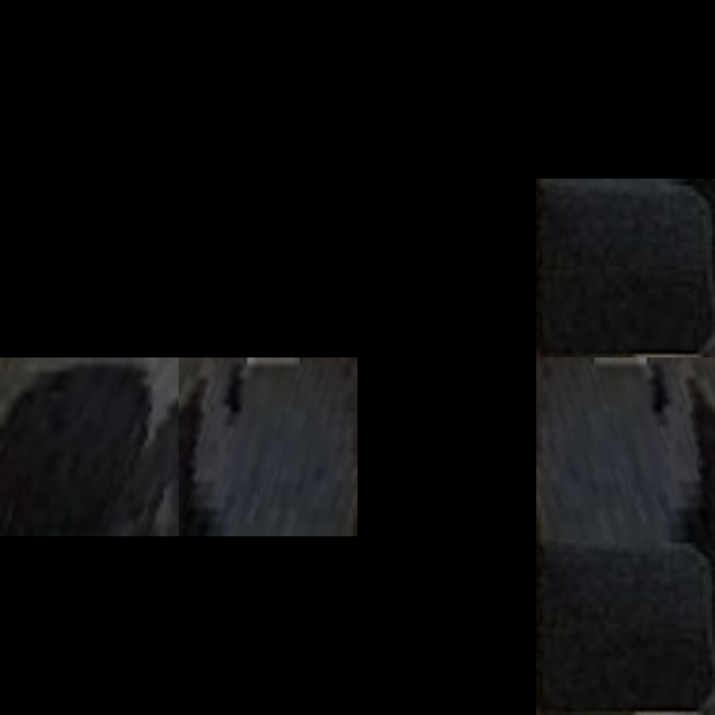
Figure 7 - Automatically-generated UV map of the bucket shown in Figure 4
As can be seen I assume that both side faces of the cube have the same texture just in opposite direction of each other and I kept the bottom face black since it is not visible in the photograph.
When user selects the object inside the photograph when required textures were extracted from the image, the object is removed from the photograph (filled with 0 instead) and a logical mask is generated. This matrix has the same size as the image and its elements are “1” if the corresponding pixels was used to be occupied by the object and “0” if otherwise. This mask matrix is used in the next section to fill the hole using texture synthesis.
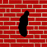
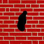
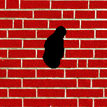
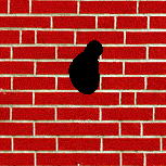
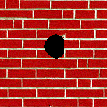
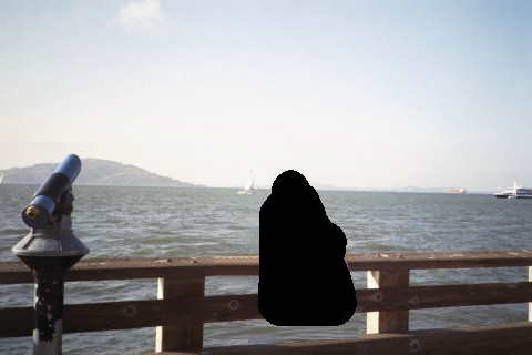
For this part of the project I used the hole-filling method described below. In this method we assume that we can guess the value of a specific pixel by knowing the value of its neighbors. For this purpose we get an NxN pixel window around the pixel in question and calculate a SSD (Sum Squared Distance) between this window and all possible pixels in the image. Note that we calculate the SSD using only the pixels that have actual values (not the ones that are a part of hole, like the following images).
![]()
Selected NxN window
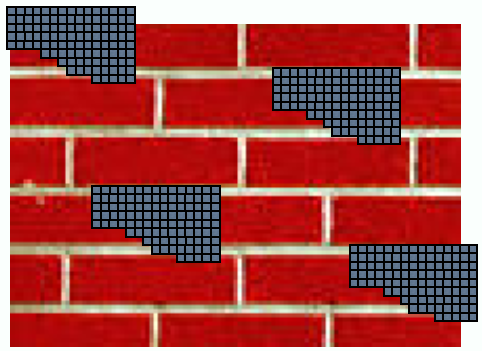
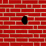
Calculate SSD for all pixels in the image
After calculation of the SSDs for all pixels, we find the minimum value of the SSD found and instead of selecting the window with minimum SSD, we use a randomly selected window with SSD value near the minimum (using a tolerance parameter) and replace the pixel in question with the center pixel of this window.
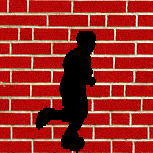
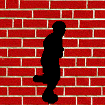
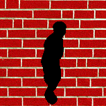
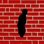
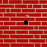
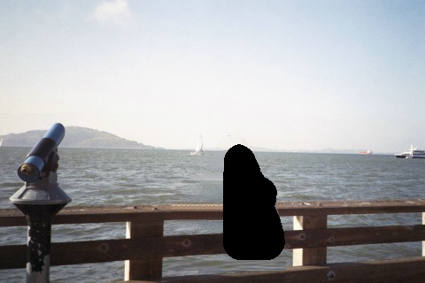
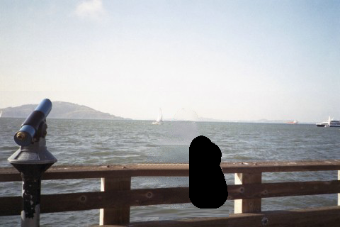
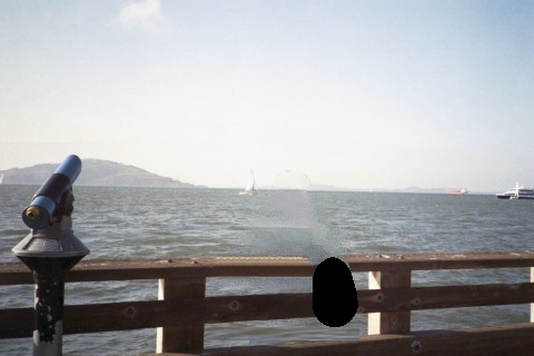
Note that this method works only if we start from the pixel with highest number of neighbors with known values. The following figures shows some results of this hole-filling method, step by step.
 |
 |
 |
 |
 |
 |
 |
 |
 |
 |
 |
 |
 |
 |
 |
 |
 |
 |
 |
 |
 |
 |
 |
 |
 |
 |
 |
 |
 |
 |
 |
From this part on, I use Blender to insert the virtual object into the photograph and simulate its physical reactions. In order to create a simple scene that simulates the physics and light effects (shadows) I used several planes as walls, ceiling and the floor and a cube as my object. Two different views of the scene created for the selected photograph is shown in the following figures.
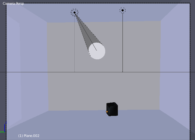
Figure 8 - Camera view of the 3D scene created based on the selected photograph
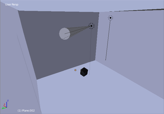
Figure 9 - Another perspective view of the 3D scene created based on the selected photograph
It makes the alignment process a lot easier if you use the original image as a background for camera view. For this matter check “Background Images” in the middle panel then use “Add Image” button to choose the main photograph as the background.
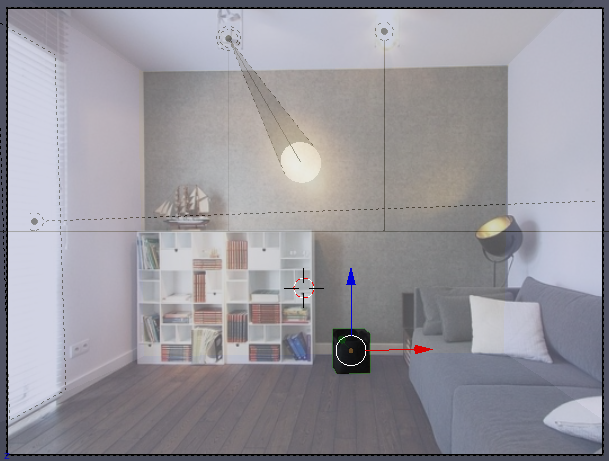
Figure 10 - Using the photograph as the background
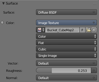
As explained before, GenerateCubeMap function provides us with a UV map for the cube that would project the same texture as the object in the photograph on the cube model. To apply this map on our model select the model (note the “object mode” option at bottom of the screen) and go to “Material” tab. Add a “Diffuse BSDF” material under Surface then select “Image Texture” as for Color and then choose the generated UV map as for image file. These configurations are shown in the following image.
To achieve better results, I inserted several light sources into the scene to simulate the lighting conditions of the scene. There are several types of light sources in Blender which can be add using “Lamp” submenu in “Add” menu at the bottom of the screen; I describe only three types that I used in this scene.
This source is like a normal light bulb, it propagates light in a spherical volume and cast shadows for object that it hits on the way. The point light in the scene in shown as (1) in the following figure. This type of light source doesn’t have many configurations, the only option that you can change about it is its strength, beside its emission color.
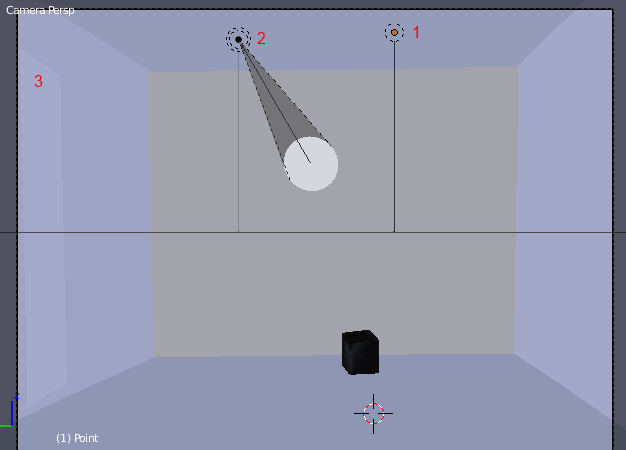
Figure 11 - Lights in the scene
The spot light of the scene is shown by (2) in the Figure 11. As can be seen, a spotlight is a directional light and works like a projector. For this light source you have to choose its strength, color and the setting of its spot shape; the angle of the light cone and how rough the light is going to blend into the scene.
Area light is a light source which is distributed on a surface, like a window or a fluorescent ceiling light. Note that if the area of the source is relatively large (which is the case here), it would generate huge amount of salt and pepper noise in the rendered image. In that case you can use a plane with emission material instead.
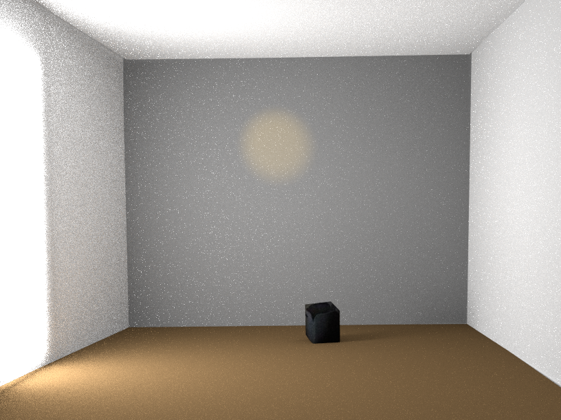
A rendered image of the created scene with lighting simulation is provided in the following figure. (Click for high resolution images)
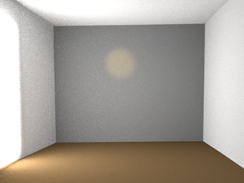
Figure 12 - A comparison between the created scene in Blender (left) with the actual photograph (right)
You can see the effect of the sunlight on the floor and the ceiling through the window and the effect of the spotlight on the back wall. Both these light sources would cast shadows to generate realistic light effects in the result. Also in order to achieve better results, the floor and the back wall have almost the same color as the original photograph.
In order to make physics simulation in Blender, our objects should have a physical body. This physical bodies could be either active, i.e. it would control the 3D mesh of the object or passive, i.e. the animation will control their movements. In our case the walls have passive bodies and our object switches between active and passive, because sometimes we want to move the object around by mouse (passive) and sometimes we want the model to have a free fall or collide with other objects (active).
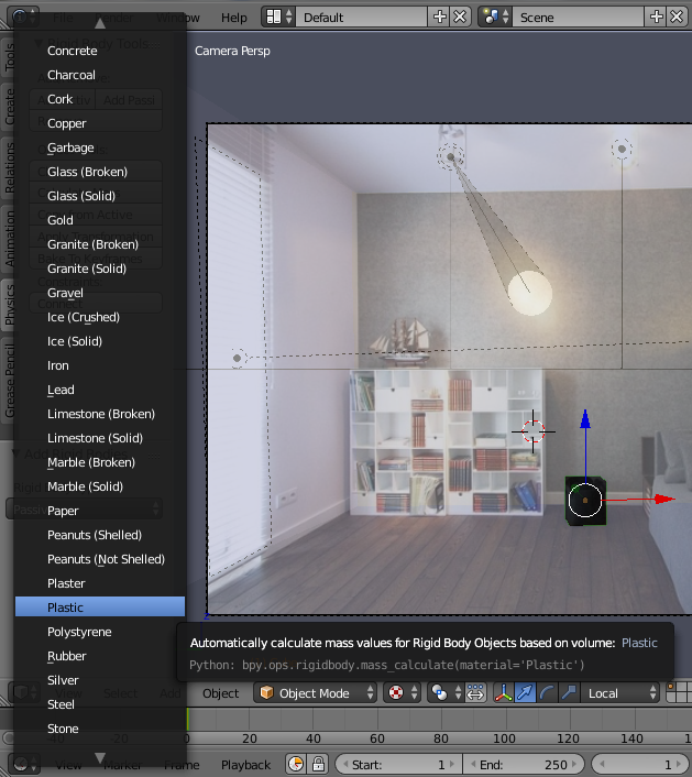
To create physical bodies for our object we select them by right click and then use “Add Active” or “Add Passive” buttons in physic tab in the left panel. We can also calculate our object mass by selecting “Calculate Mass” button. This button will show you a list of different materials (iron, plastic etc.) to choose from and then it would calculate the total mass of your object according to your choice. The objects with zero mass wouldn’t budge under any circumstances!
The main idea of the animations in Blender are the keyframes, certain frames in which you want your object to have a certain situation e.g. specified position, rotation, scale, the fact that the physical body is active or not, etc.
To insert a keyframe, after changing the situation of the object as we want (position, rotation etc.) we press “I” key and select the type of keyframe that we want. If we choose “Location” it shows that we want our object to end up at that exact position even if the physics simulation wants our object to be somewhere else, on the contrary if we choose “Visual Location”, Blender knows that we want our model to move freely by the laws of physics.
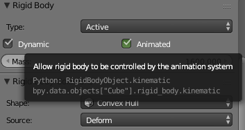
At last if we want our object to switch from passive movements to active, we have to change the state of “Animated” switch in Physics tab in the right panel, then we can insert a keyframe with this new state by right click on the checkbox button and select “Insert Keyframe”.
 |
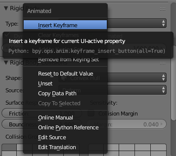 |
Figure 13 - Switch between Active and Passive mode in the middle of animation
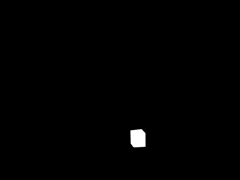
For get better result we insert our virtual object into the photograph using an alpha blending. For that purpose we need to create an object mask. The mask has the same size as the rendered image and its elements would be greater than 0 at pixels where inserted objects exist, and 0 otherwise. To generate this mask save your scene under different name and open it up (e.g. room4-mask.blend).
First of all, switch to “Blender Render” instead of “Cycles Render” then remove all materials of all objects in the scene. Select the cube, add a “Diffuse” material and set the color and intensity to 1, then select “Shadeless” under Shading. Repeat this for all other objects (walls, floor etc.) expect that change intensity and color of these objects to 0. At last change the “Horizon Color” to black in Scene tab.
After that if we render our scene we would see something like this:
We now blend each frame using the equation below in Matlab:
composite = M.*R + (1-M).*I + (1-M).*(R-E).*c
Where,
M: Black and white Mask
R: Fully rendered frame
E: Our empty 3D scene rendered image (Figure 12)
I: Our background image
C: Controls the strength of lighting effects of the inserted object (shadows, caustics, interreflected light, etc)
The separate parts of first frame of my result is shown in the following figure (Click for larger images):
|
|
 |
|
 |
I (object deleted) |
E (empty scene) |
R (rendered scene) |
M (alpha mask) |
Result (object inserted) |
A quick review of this approach is shown in this video:
This is just a test scene that I obtained during my work:
You can see the final result here:
In this video the original photograph smoothly morphs into our synthesised one, then our object starts to fly around in the room. You can see the bloom effect (light rays) of the bright window when the object is in front it, the shadows cast by the spot light on the back wall is also interesting.