The main purpose of this assignment is to generate a panorama image, stitching several individual images, manually and automatically. In manual method, user has to select several interest points in each pair of images but in automatic mode, these points are selected automatically using Harris corner detection method (using several filtering method which I will describe later).
The algorithm should be able to calculate the homographic transform required to warp each image into a specific projection. In this project I preserve the projection of the main image (central image) as panoramical projection and then warp all other images into this projection.
During this project, Harris corner detection was used as feature point selector along with “Adaptive Non-Maximal Suppression” and 1-NN/2-NN thresholding to filter the result of this method, all of which will be explained later in this report.
The following steps should be done in order to generate a panorama image manually:
For this step I wrote a simple tool using matlab function ginput. Using this tool user can select unlimited number of points in an image set and press Enter key at the end to finish this process.
In the following figure, manually-selected points in an image pair are shown:

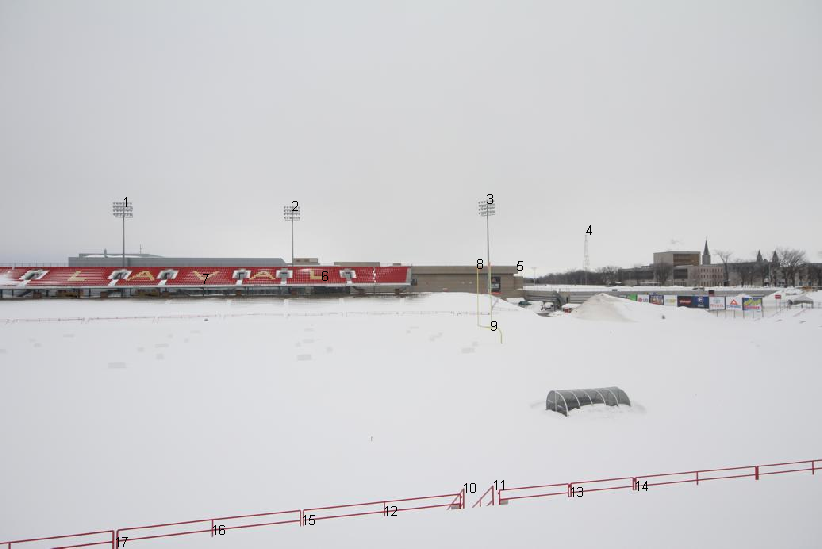
As can be seen user has selected 17 points of interest in both images. This step was done for all images in this image set.
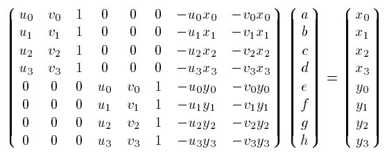
The only part of the manual approach that needs explanation is calculating H using least square approach. For this part, the algorithm solves a linear matrix equation to calculate H.
For homography we have:
![]()
Where ![]() is a point in the reference image and
is a point in the reference image and ![]() is a point in the image that we want to warp. In order to calculate H we have to solve the following equation:
is a point in the image that we want to warp. In order to calculate H we have to solve the following equation:

As mentioned before there is no limit in number of x and x' points to select, as a matter of fact, the more selected points, the more accurate results.
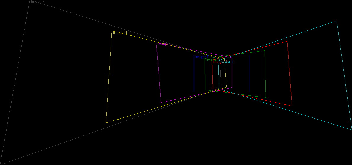
After calculating H, I used an inverse transform to warp the input images into a panoramic projection. In order to do an inverse transform, first we need to calculate the position of the image corners after transformation. For this part we have to use a forward transform using H and then we should calculate the inverse matrix of H for the rest of the procedure.
I calculate an axis aligned bounding box for each image which needs to be transformed. Iterating all pixels of these bounding boxes, the algorithm perform an ![]() transform on the pixels to obtain their color using an interpolation on the source image. Then I stitch these boxes together to generate the result.
transform on the pixels to obtain their color using an interpolation on the source image. Then I stitch these boxes together to generate the result.
The structure and the final image is shown in the following figures (click for larger images):
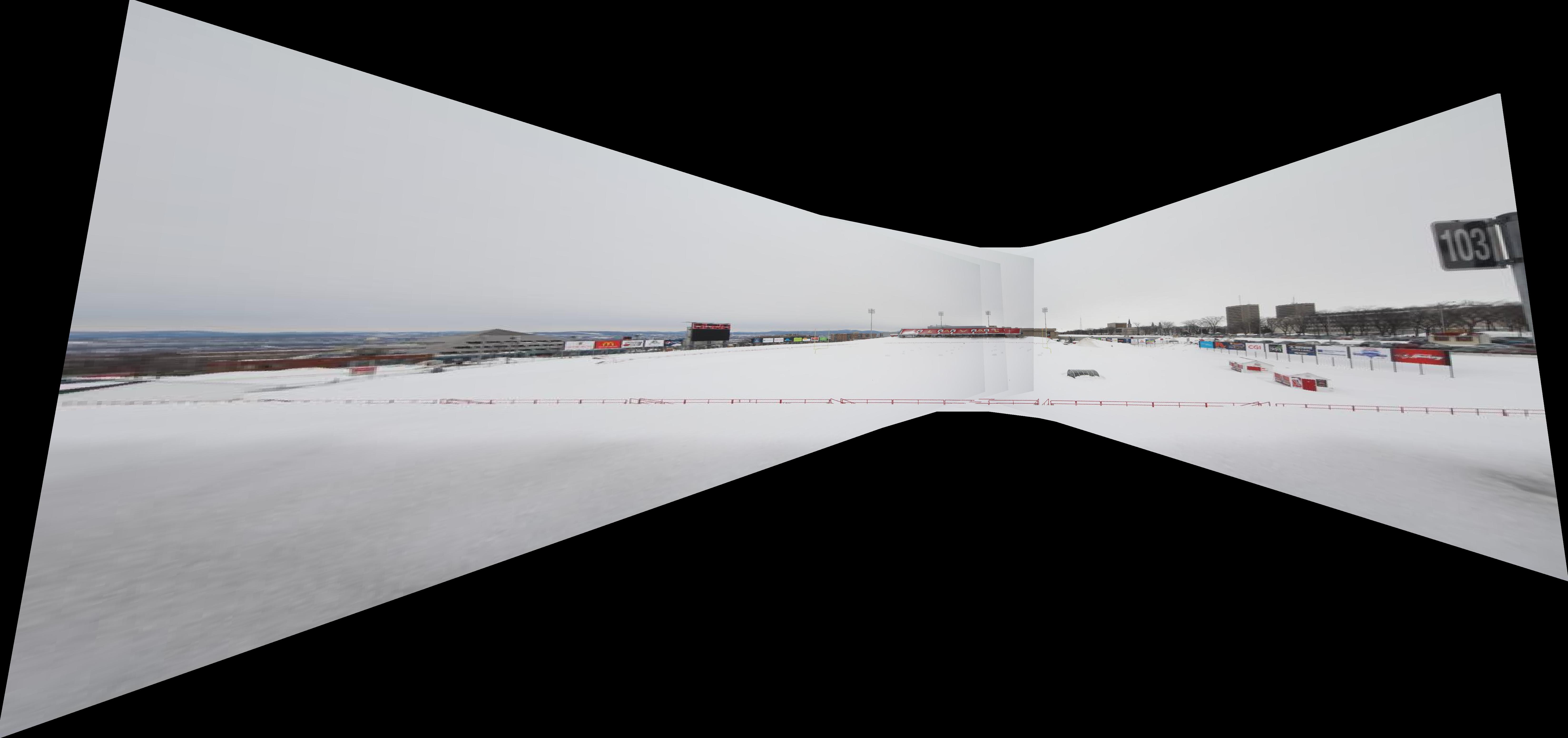
Non-cropped result of the manual approach
In this step, we should stitch the warped images in order to generate a panoramic mosaic. It is possible to rewrite pixels on eachother on overlapping parts but this will generate edge artifacts in the results (as can bee seen in the above figure). To avoid the artifacts, I simply put the maximum value calculated for overlapping pixels, however it is possible to use other blending methods like alpha blending (weight averaging) with alpha = 1 on the center of the image and alpha = 0 on the edges.
Here are the final results of the manual approach with and without blending. Note that the results are automatically cropped not to contain the black parts: (Click to see larger images)
 Manual approach result without blending (Automatically cropped)

Manual approach result with blending (Automatically cropped)
In this approach, the algorithm should be able to act completely automatically. The only part that was done manually before was feature point selection. In the automatic approach we use Harris corner detection to select the points of interest.
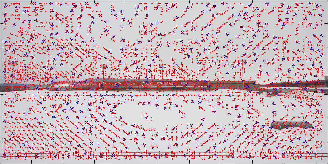
As can be seen this method detects lots of points which would result in very noisy and unacceptable results. In order to filter the detected corners, we used the method describing in [1]. In this article an “Adaptive Non-Maximal Suppression” method is described in which, corners are sorted descendingly by their distance from their closest more powerful neighbor corner. Then a specific number of these corners are selected from the top of the list.
In the following figure, 500 selected corners by this filtering method are shown (red points are all corners detected by Harris; the selected ones are distinguished by blue circles):
After selecting our points of interest now we have to compare them one by one in order to find best matches. The usual way to compare two points is to compare the specifications of them and their neighbors, i.e. their feature descriptor. In the above mentioned article, the authors suggest to use a discrete wavelet transform (using Haar) of resampled 8x8 pixel window as a descriptor for each point. This window is generated by resampling every other 5 pixel, from a 40x40 window around the point in question. It’s also mentioned that this patch should be normalized to have maximum absolute intensity value of one and mean value of zero.
The following figure shows the extracted windows (before and after normalization) :
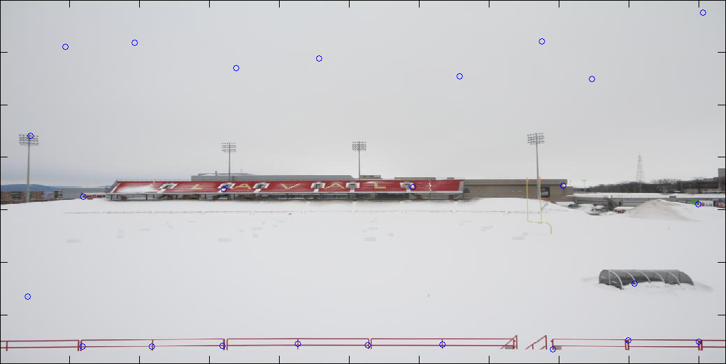
25 Selected points by Harris and ANMS
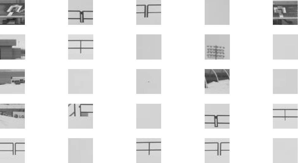
Corresponding 40x40 windows (descriptor pathes)
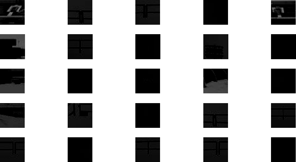
Descriptor patches after normalization
As can be seen, normalization would make our descriptor invariant to affine changes in intensity (look at patches selected from different parts of the sky).
We use nearest neighbor approach to match the descriptors extracted from main image points with the points of the image to be warped. This means that we calculate the Euclidian distance between a descriptor from first image and all the descriptors from the second image to find the closest matches.
In the article a specific thresholding method is discussed that allows us to eliminate most of the incorrectly selected matches for our purpose (generating panoramic images). This thresholding is performed on 1st nearest neighbor distance to 2nd nearest neighbor distance ratio (1-NN / 2-NN). According to the article the best result would be achieved with a threshold between 0.4 and 0.6.
The following figure shows the effect of this threshold in point matching, comparing matched points between two consequent images, using thr=0.4 and thr=0.5:
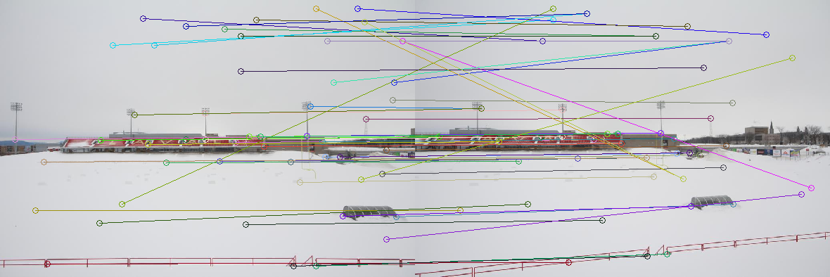
Strongest 250 with ANMS, 1-NN/2NN < 0.5
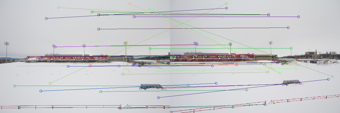
Strongest 250 with ANMS, 1-NN/2NN < 0.4
RANSAC is an iterative method to estimate parameters of a mathematical model from a set of observed data which contains outliers [2]. Here we use RANSAC to estimate H (our mathematical model) using 4 matched points from source and destination image (observed data) comparing our result with counting our non-aligned points after performing the calculated H (outliers). RANSAC is an iterative approach in which we generate a different mathematical model using randomly selected input data in each iteration. We count the number of our inliers (or outliers) of each model in order to find the best model generated.
Here, in each iteration we perform the calculated H on all detected points in the first image. To count our inliers we use a distance threshold that specifies if a point is transformed correctly on its corresponding point in the second image or not. After selecting the best model of homographic transform matrix (H), we calculate it again, this time using all inlier points to achieve better results.
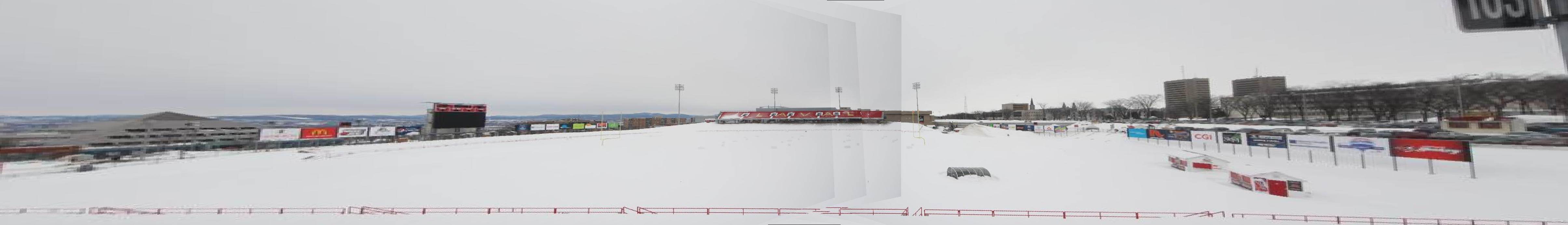
The last step of the automatic approach is the same as the manual approach, we stitch images together to generate the results. Here are the results: Note that the result is automatically cropped (Click for larger images)

Panorama 1 - PEPS (Laval University)

Panorama 2 - Caféteria (Alexandre-Vachon Building, Laval University)

Panorama 3 - Adrien-Pouliot and Alexandre-Vachon Buildings (Laval University)

Panorama 4 - Beautiful skyline of Montreal
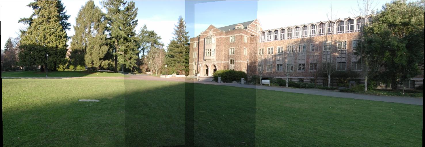
Panorama 5 - Campus of University of Wisconsin - Madison
As can be seen, in the last two examples, input images have noticable difference in lighting which produce edge artifacts in the output.
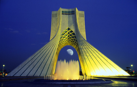
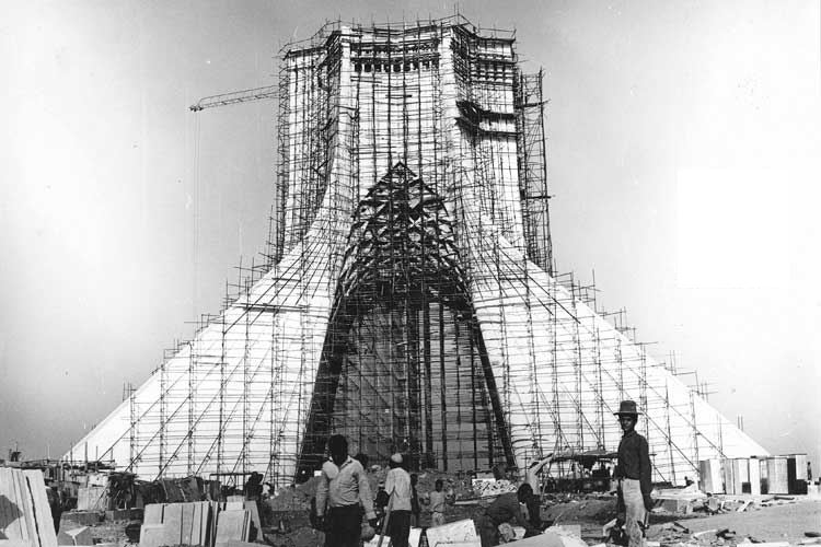
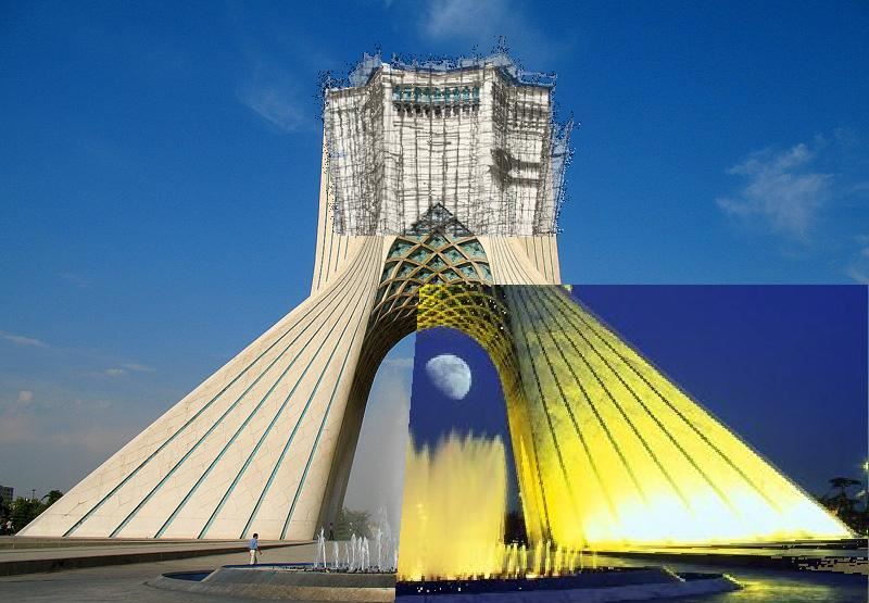
We can combine two or more images using the same idea as described above. Here are some examples:
 |
 |
 |
 |
||
Combination of images (Example 1) - Azadi square, Tehran
 |
 |
 |
|
Combination of images (Example 2) - Egyptian pyramids, Cairo