Final Project: Poisson Image Editing

This project implements the seamless image composition algorithm from Pérez, et al."Poisson Image Editing" [1] . Given a source image, a target image and a "mask" image to determine which pixels should blend from the source image into the target image. A simple cut and paste of the masked region gives a bad blend since the gradients of the source do not match the gradients of the target. Given that people often care mush more about the gradient of an image than the overall intensity. Therefore, we compute information about the gradient for each pixel in that part of the source image, and then apply the same gradient in the target image. The result is that each "transplanted" pixel on the target image has a gradient that is the same as the gradient of the corresponding pixel on the source image, but still have all the features of the source image.

1. Algorithm Details

1.1- generating the matrix A:

The image blending problem is phrased as a least-squares problem, which requires solving AX = B for every pixel under the mask.
We have a mask which has the same size as both the source and target images. The mask's values are either 0 or 1. In our final image, if the mask's value is 0, we want to just take the target's pixel value at that point. If it is 1, we want to set up a linear equation such that the gradient for a given pixel is the same in both the source and final images.
We go through the entire image and create a vector with one entry for each pixel which takes the actual values of either the target image, if the mask was 0 at that point, or the gradient value from the source if the mask was 1 at that point. Once we have the coefficient matrix A and B, we can find our output image.
B is a (Nx1), represents the desired output gradient and values, and A is a large, sparse matrix define as (NxN), represents unknown gradient values. A is same across all color channels hence we create is only once, but we calculate three different B column vectors: one for each color channel. X contains the coefficients of each output pixel in X. The value of N is the number of pixels that are under the mask and has 1 value.

1.2- Border detection:

For the pixel that was not in value 1, like some positions that were under the mask, than I gave the correct value(4 if not the border). But, the problem arises when the pixel is on the borders which may not match the gradients that existed in the source image. To handle this problem, the Laplacian is used on each pixel in the source image:
4(Source-pixel) - (Up-Neighbor) - (Down-Neighbor) - (Right-Neighbor) - (Left-Neighbor)

2. Mixed Gradient

Follow the same step as poisson blending but use the gradient in source or target with the larger magnitude, rather than the source gradient. One possibility of blending using mixed gradient is to blend a picture of writing on a plain background onto another image.

3- Result of Poisson Blending:

3.1- First Blending :

3.1- Inputs

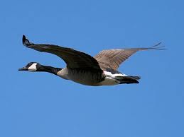
3.1- Output

1.3.2- Second Blending :

1.3.2- Inputs

1.3.2- Output

3.3- Third Blending :

3.3- Inputs

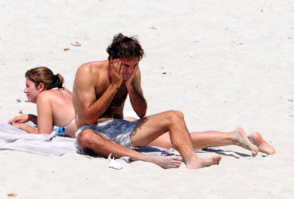
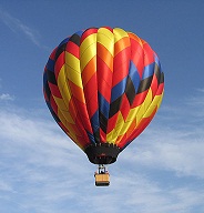
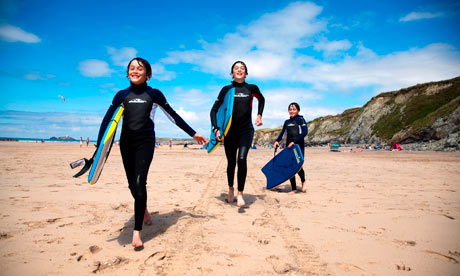
3.3- Output

1.3.4- Fourth Blending :

1.3.4- Inputs

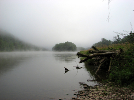
1.3.4- Output

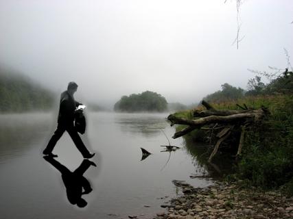
1.3.5- Fifth Blending :

1.3.5- Inputs

1.3.5- Output

4- Result of Mixed Gradient:

4.1- First Blending :

4.1- Inputs

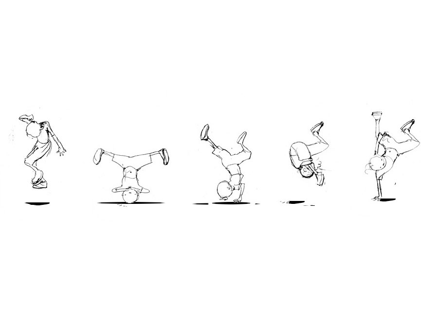
4.1- Output

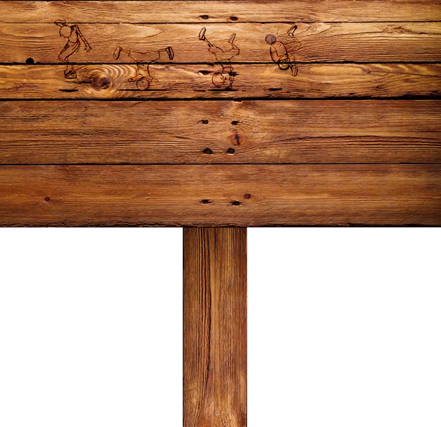
The first image is resulted by Poisson blending and the second one is the result of the Mixed Gradient.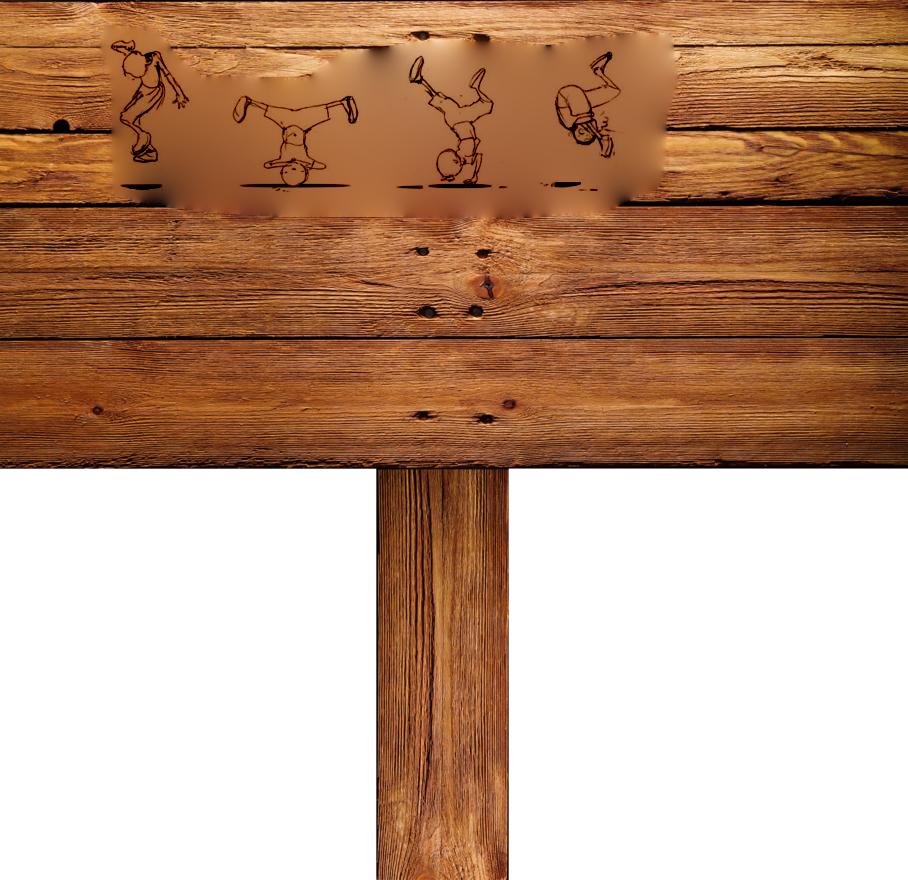

4.2- Second Blending :

4.2- Inputs

4.2- Output

I manually croped the result.

4.3- Third Blending :

4.3- Inputs

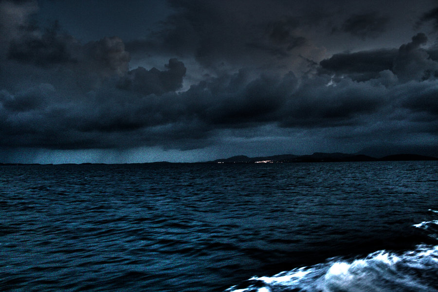
4.3- Output

4.4- Fourth Blending :

4.4- Inputs

4.4- Output

5- Faild Result:

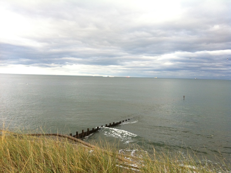
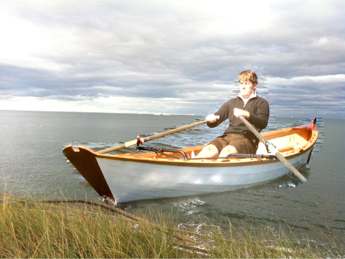
The method fails when the gradients close to the seam are too different. For example, when a constant region is merged with a non-constant one as in the images below. Even though both original images have similar colors, the result does not look as a true picture.

5.1- Inputs

5.1- Output

5- Color2gray:

Using the mixed gradient method, we can create a gray image that has similar intensity to the rgb2gray output but has similar contrast to the original RGB image. This is done on the HSV color space. The intensities in the V-channel is to be preserved, but at the same time it needs to respect the contrast. The S-channel serves as a good guidance for contrast since the digit has different color compared to the background and it stands out in the saturation channel. Therefore, we can treat the V-channel as the target image and the S-channel as the source image in the mixed gradient blending.

6- Texture Flattening:

The idea is to only keep gradient information where there's a sharp edge, and to zero out the gradient everywhere else. This way, only the sharpest edges will be transferred over to the new image. I tried Canny Edge Detector to find the edges.
Unfortunately , I needed more time to remove the bug of my code !! :(