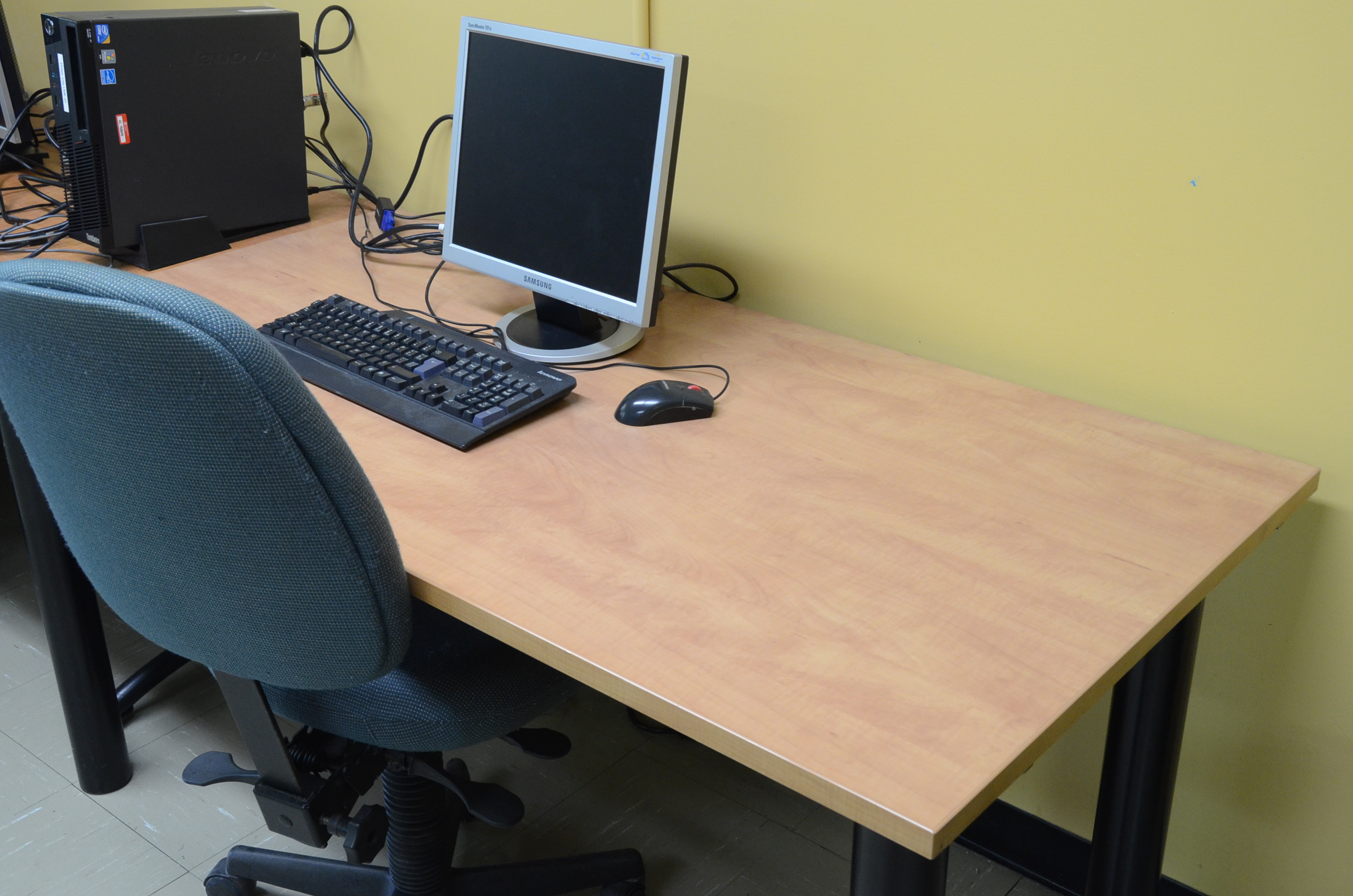
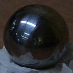
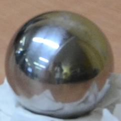
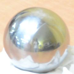
Subsets of the scene, displaying the spherical mirror at three different exposures, were taken in order to calculate the irradiance map:
| t = 1/160 | t = 1/40 | t = 1/10 |
| 
| 
|
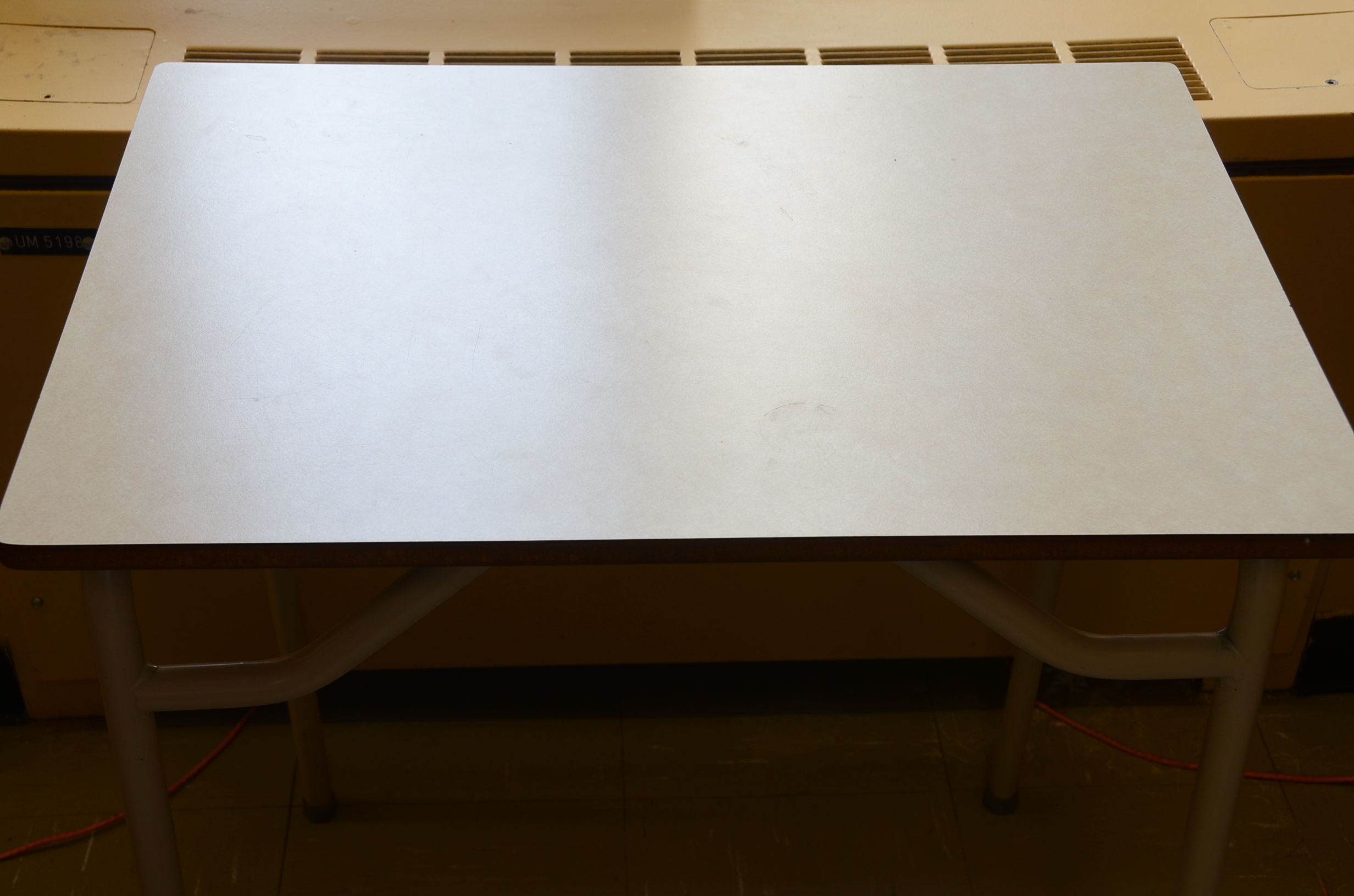
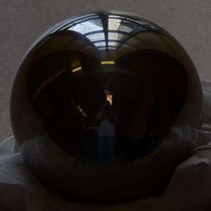
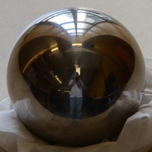
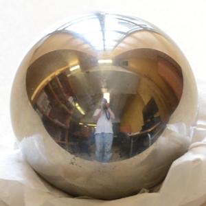
Again, subsets of the spherical mirror at three different exposures were taken in order to calculate the irradiance map. The window can be seen on the spherical mirror:
| t = 1/250 | t = 1/60 | t = 1/15 |
| 
| 
|
Part 2: Converting these exposures into a single HDR radiance map
Methods In order to get high dynamic range (HDR) images for the illumination from the low dynamic range (LDR) images capturing the spherical mirror, the LDR images of the spherical mirror can be combined. The basic formulas are given by Debevec and Malik 1997. The fundamental idea is, that value Z of pixel i at exposure j equals:
Z_ij = f(E_i x t_j) (Eq.1)
where E_i denotes irradiance and t_j shutter time. f is an unknown function describing the response function of the image sensor and has to be determined from the acquired set of images. This was done using the algorithm provided by Debevec and Malik 1997:
1. chose a random selection of 100 pixels in the images showing the spherical mirror. This step
is performed in order to reduce calculation time. It is
important, however, that the three images overlap in order to select the same pixel at each
exposure.
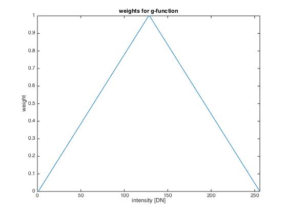
2. a weighting function was defined to weight the pixels in computation of the sensor's response
function. The goal, thereby, is to suppress saturated pixels (i.e. pixels with values either 0 or 255 where ascribed
a weight of 0) while pixels in the middle of the value range should get the maximum weight (i.e. 1).
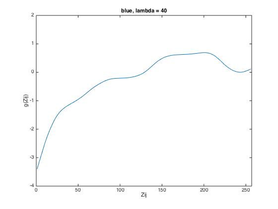
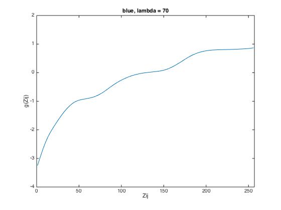
3. lambda has to be chosen, which smoothes the retrieved response function. The aim is to achieve a
response function constantly increasing. However, selection of lambda has to be done iteratively by
evaluating the computed response function.
4. calculate the sensor's response function deploying the algorithm by Debevec and Malik 1997 and
utilizing the set of randomly selected pixels from all exposures, information on shutter time,
the weighting function and lambda. Strictly speaking, the function we obtain here is not identical to
f from Eq. 1 as logarithms of E and t, respectively, are used in the calculation. Therefore, it is
denoted as:
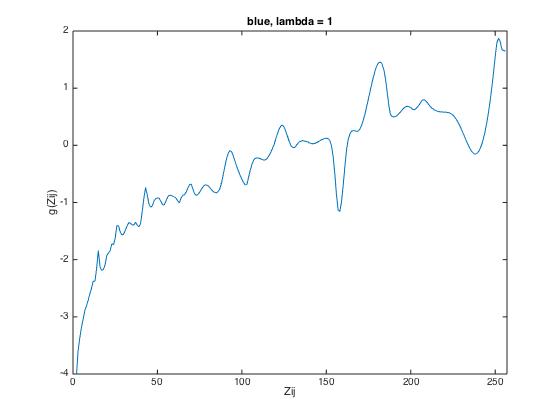
g(Z_ij) = ln(E_i) + ln(t_j) (Eq.2)
Once the sensor's response is given, the HDR image can be calculated. To do so, E_i from Eq.1 are summed up
for all available exposures. E_i for a single LDR can be retrieved via the computed g-function, as g-function
allows to look up the sum ln(E_i) + ln(t_j) from Eq. 2 for each pixel value Z_ij.
As t_j is given, E_i can be calculated.
To sum up E_i, the same weighting function as
for calculation of g was deployed in order to suppress saturated pixels.
The retrieved HDR image stores pixel values larger than 255, thus, dynamic range is enlarged.
The HDR image of the spherical mirror can directly be used as input in Blender in Part 3 where
it is used as information on illumination direction and strength in the scene.
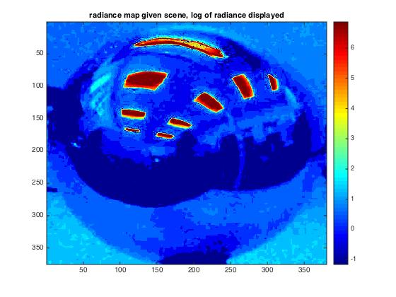
To get information on radiation, however, a radiance map can be created by just showing the HDR
image using a colormap indicating the pixel values. I did this based on the logarithm of the
actual radiance.
Results and discussion
weighting function
As described, the pixel values are weighted for the calculation of g as well as for the later inversion
of the g-function to compute radiance E. For both proceedings, the following weighting function was introduced
into calculation:
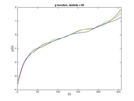
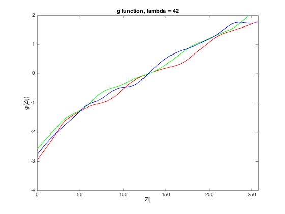
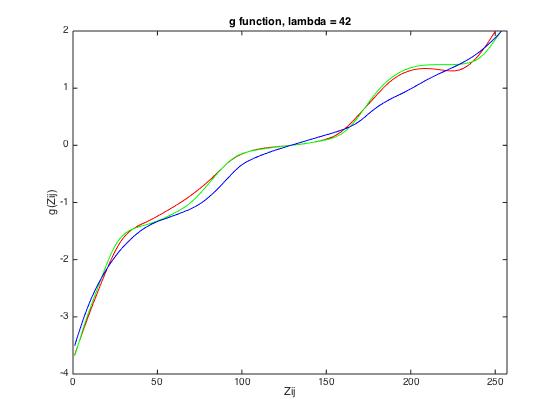
g-function
The g-function is sensor-specific and has to be retrieved for each scene. Furthermore, as a random
subset of pixels was selected, the g-function might slightly vary if it is recalculated using a different
set of pixels.
The following results show the derived g-function for the given data set (left), for scene 1 (middle) and
for scene 2 (right).
| given data | scene 1 | scene 2 |
| 
| 
|
| lambda = 1 | lambda = 40 | lambda = 70 |
| 
| 
|
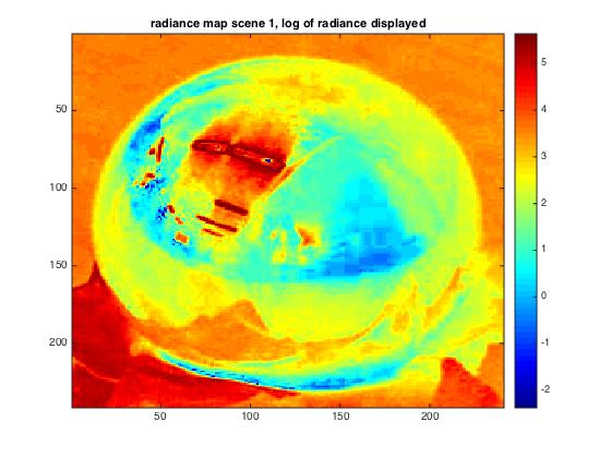
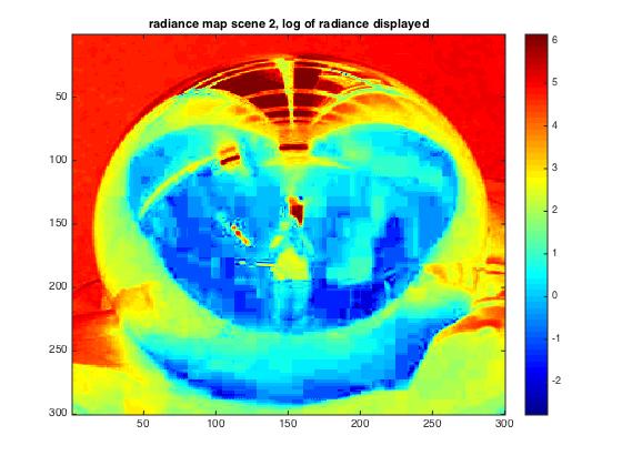
Finally, the radiance maps look as follows, where radiance is mapped as logarithm of measured radiance:
| given scene | scene 1 | scene 2 |
| 
| 
|
As visible, differing amount of radiance can be recognized, for example between the less illuminated scene 1 and scene 2 where illumination is higher due to the window. In general, light sources can clearly be recognised as red colors.
Part 3: Rendering synthetic objects into photographs
Methods
To add objects into existing scenes, three properties have to be adjusted for each object, namely
its orientation, illumination and shadowing.
As rendering of the scenes was done in Blender, orientation is controlled manually. For
a correct illumination and shadowing, the calculated HDR images are introduced into Blender.
This subsequently allows for an appropriate rendering of the illumination conditions.
To reconstruct the scene, three renders were calculated for each scene:
1. R: the scene containing all objects. R consists of a local scene model representing the desk
surface in our case, and the objects. For rendering R, illumination, shadows and reflections onto
the modeled plane caused by the objects are computed.
2. E: render of the empty scene, representing a local scene representation. This model later
is subtracted from the render form step 1 as we do not want the local model scene within the
final result. The reason for this is, that we want to use actual surface captured by the background image
and only add shadows and reflections to the plane.
3. M: a mask for the objects.
These three render R, E, M and the background image I, comprising the actual scene to which the objects are added, are combined in Matlab using the formula:
M.*R + (1-M).*I + (1-M).*(R-E).*c (Eq. 3)
where c has to be chosen appropriately.
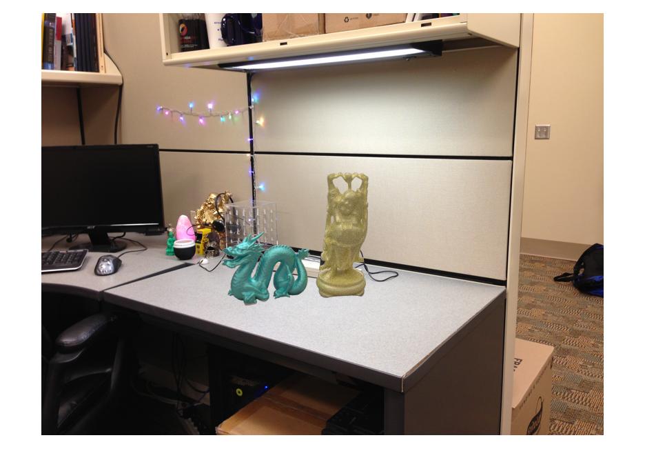
Given scene
To test the processing, I followed the tutorial using the given scene. Here, I placed two objects,
namely the dragon and the buddha, into the scene, where properties of the buddha were set to subsurface scattering and a
yellowish color while for the dragon, I chose Glossy BSDF with a Beckmann distribution as surface
property and chose cyan as color. For the illumination, the provided HDR was used.
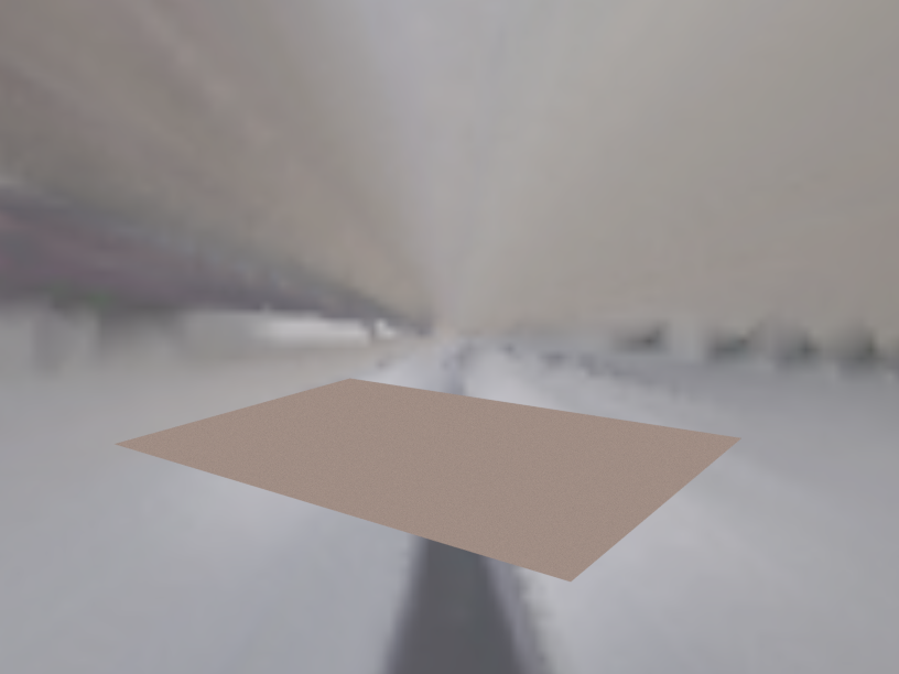
Then, the three renders R, E and M were computed:
| render with all objects, R | render of empty scene, E | render of objects mask, M |
| 
| 
|
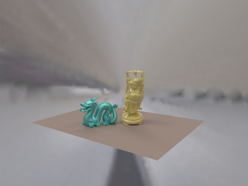
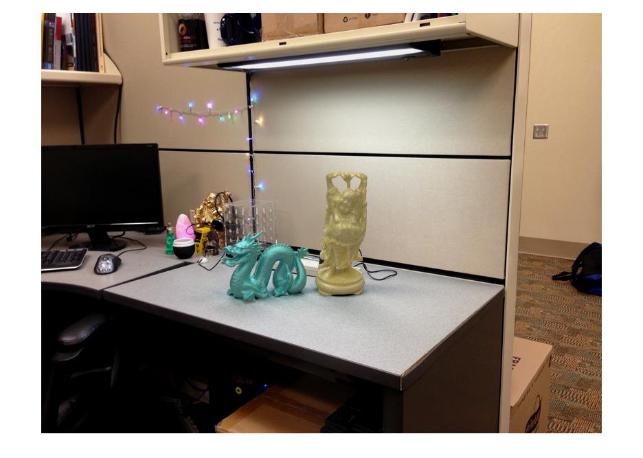
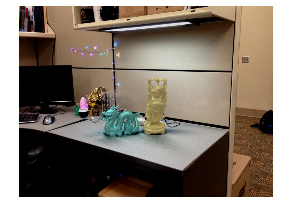
Combination of these renders with the background, according to Eq. 3, results in following results, depending on chosen weight factor c:
| final result with c = 0.1 | final result with c = 2.5 | final result with c = 5.0 |
| 
| 
|
As visible, c controls the shading of the objects within the scene, while shading the inserted objects themselves remains unaffected. If c is set too small (left), the inserted objects do not fit well into the scene but seem unnaturally lift. If c is too large on the other hand, the shadows are too strong compared to the shadows from the objects present in the original scene (right). However, if c is set appropriately, the objects fit well to the scene. For the given scene, a value of c=2.5 was considered as good choice (middle).
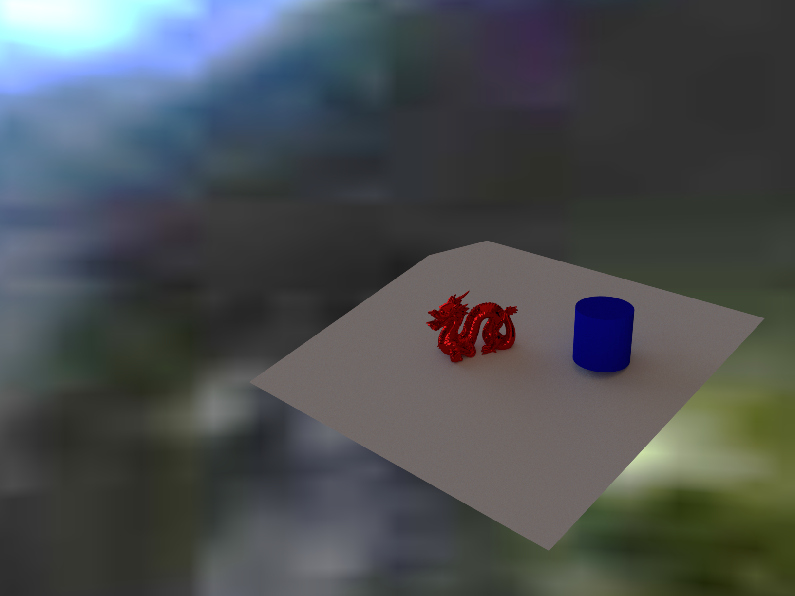
Scene 1
Processing of the own scenes follows exactly the same principle as described in the methods.
The HDR computed for scene 1 based on the spherical mirror was introduced to blender as
information on illumination conditions.
In the first of the two own scenes, I inserted an additional object (the cylinder) not present in the given scene, as
requested. For the cylinder, I chose a blue color and Diffuse BSDF surface scattering. To allow
for a comparison, I again added the dragon, this time with red surface and Sharp Glossy BSDF
reflectance properties.
Renders of the three intermediate steps for R, E, M are the following:
| render with all objects, R | render of empty scene, E | render of objects mask, M |
| | 
|
The final results for different values for c:
| final result with c = 0.1 | final result with c = 3.0 | final result with c = 5.0 |
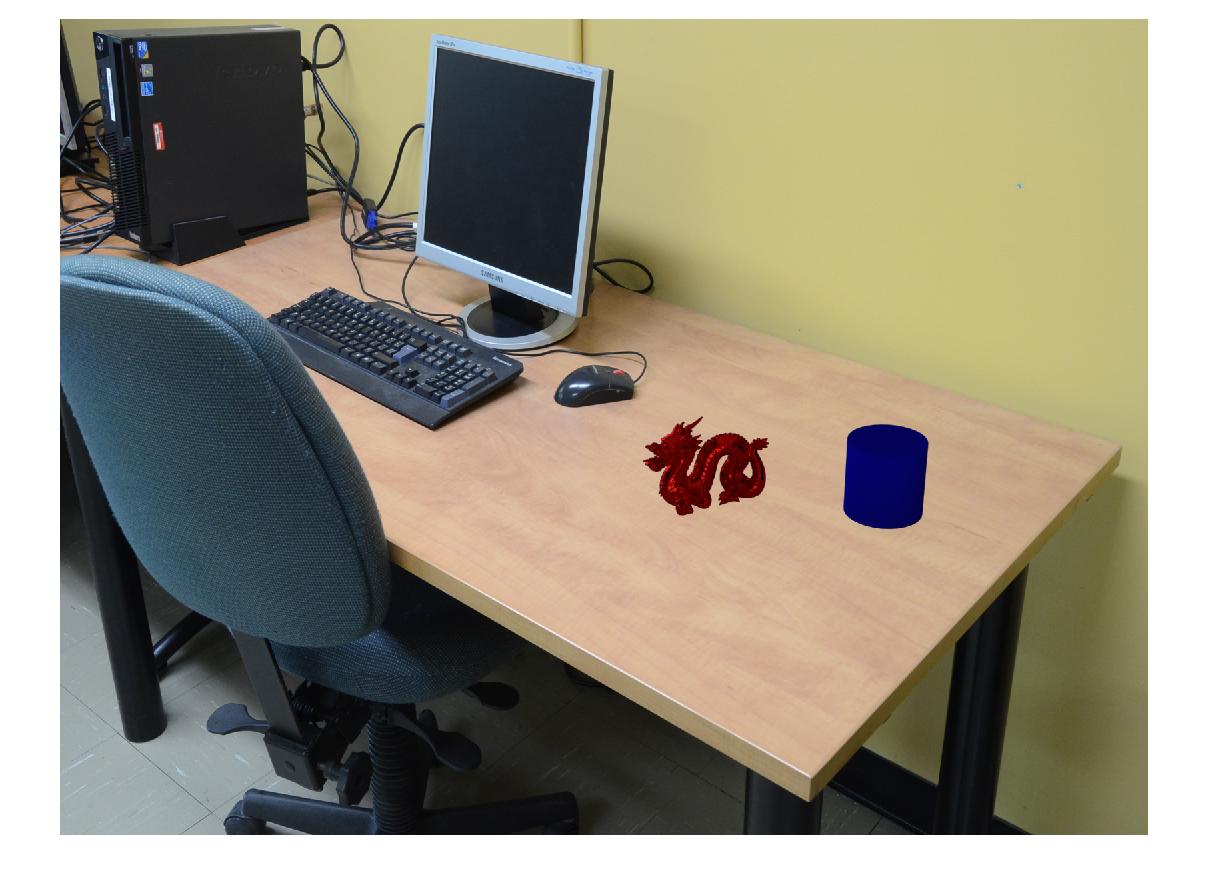
| 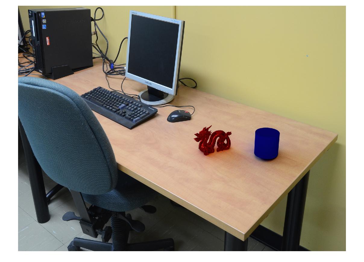
| 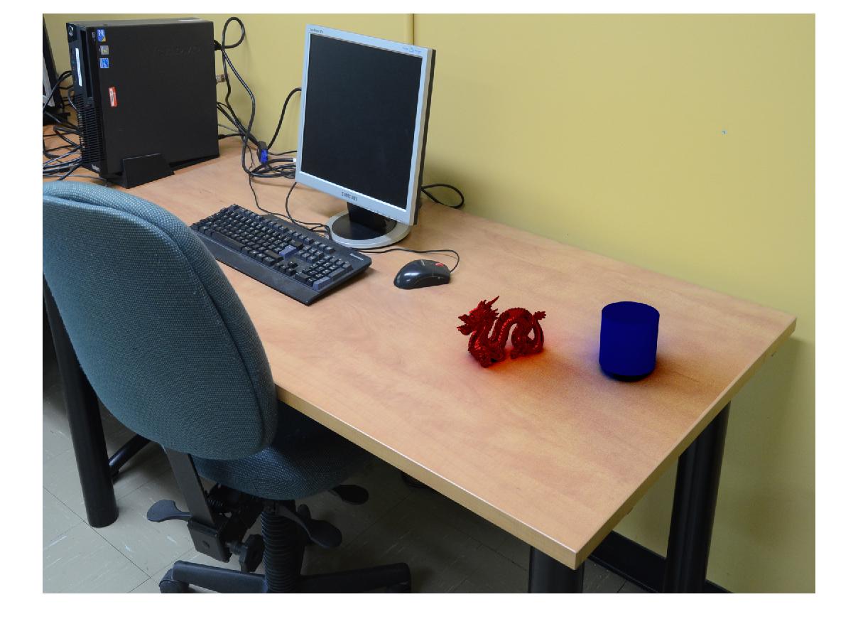
|
Here again, c=5.0 seems a bit too large (right image) while c=3.0 seems to lead to a more pleasing result. Scattering conditions become visible here as the objects reflect some colors onto the table. This effect, as the shadows, is stronger with increasing c-values.
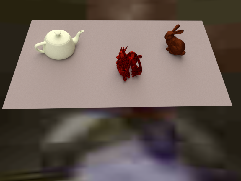
Scene 2
I placed 3 objects into scene 2: First a brown rabbit with GGX Glossy BSDF surface properties, second
a red dragon with Sharp Glass BSDF scattering and third a somewhat yellowish teapot with Diffuse BSDF
surface characteristics.
Renders of the three intermediate steps for R, E, M are the following:
| render with all objects, R | render of empty scene, E | render of objects mask, M |
| | 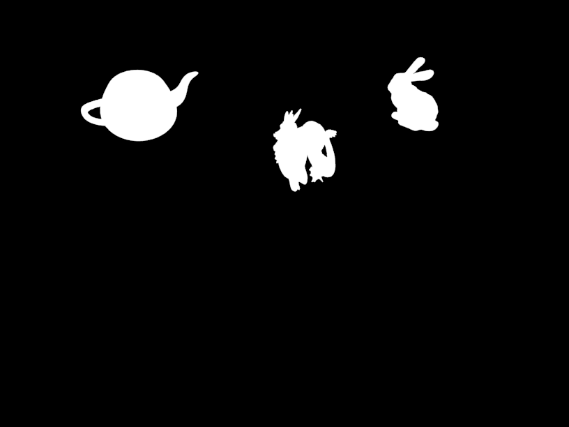
|
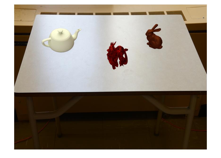
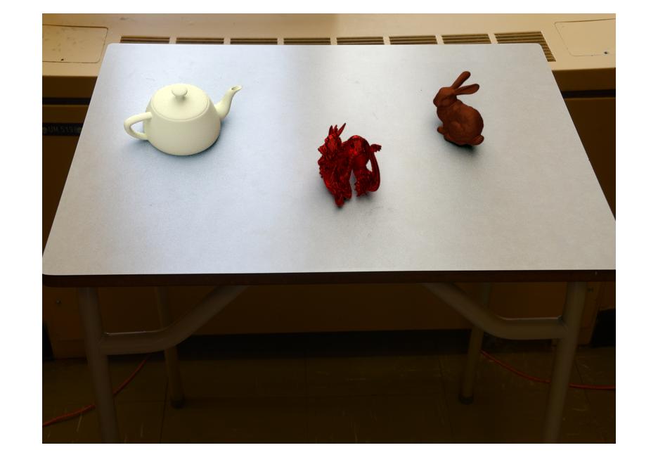
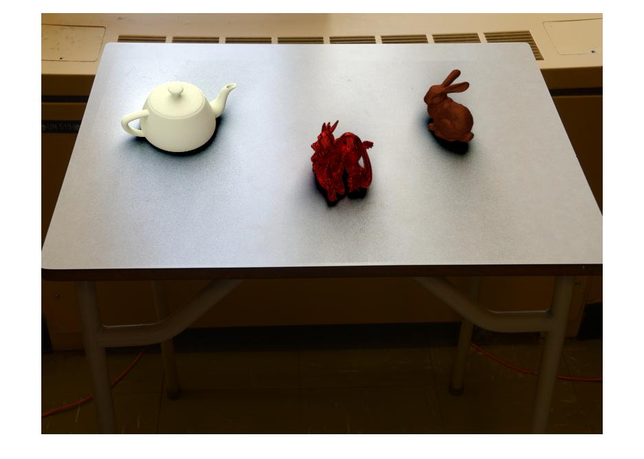
The final results for different values for c:
| final result with c = 0.1 | final result with c = 2.0 | final result with c = 5.0 |
| 
| 
|
For this scene, I consider c=2.0 as good selection. In this scene, the strong backlight conditions
are well represented in the scene. Backlight is the reason why the objects appear that dark.
In this scene, importance of orientation becomes apparent as the dragon reveals a rather unnatural attitude.
Concluding remarks
One difficult task in the processing is correct alignment of the plane, which models the environment
in the background image. This plane has to be well aligned to the plane onto which one aims at inserting the
objects in order to get a visually pleasing result.
Another aspect affecting the visual quality of the final result is the resolution with which the rendering
is performed. The given scene and scene 2 were rendered with 25% of the original resolution,
what took up to 2 minutes per frame. Scene 1 was rendered at 50% resolution, what took 4-5 minutes
per frame. On the other hand, rendering at full resolution would have taken more than 10 minutes. The salt-and-pepper-noise-like
artifacts in the renders might result from this reduced resolution.