Warmup
In the warmup section, the algorithm for image warping as used in all subsequent parts is developed.
The algorithm applies a homography on an image and returns the transformed image.
The algorithm works as follows:
1. apply homography on image corners in order to determine outline of new canvas
2. span new canvas of required size as found in step 1.
3. perform backward-transformation
In order to apply the homography, all image coordinates were transformed into homogenous
coordinates. A main issue arises from the transformed corners resulting possibly in negative
coordinates. The new canvas, thus, was transposed in order to obtain positive coordinates only.
However, transposition has to be kept in mind for subsequent backward-transformation where for
every pixel in the new, transposed canvas, coordinates in original image are calculated
applying the inverse homography and respective intensities are interpolated from the original image.
Result of applied homography looks as follows:
Part 1: Manual matching
Methods Manual matching consists of four steps:
1. Features matching
2. Computation of the homography
3. Warping of images using the homography
4. Image blending in order to retrieve a mosaic
In part 1, feature points were selected manually (part 1). This makes the entire process much easier as
8 points as required to compute the homography are selected by visual comparison of the images.
This directly results in a matching set of features for two images.
Based on the selected matches, the homography can be computed. The idea is to establish a
system of equations as Ah = b where A stores the coordinates from image 1, h the elements of the
homography and b the elements of image 2. This would need 4 points only. However, in order
to make homography estimation more robust, 8 points were used for homography estimation.
To solve the system of equations, the problem can be reformulated to Ah = 0, where A is
filled as:
-x_I1 -y_I1 -1 0 0 0 x_I1*x_I2 -y_I1*x_I1 x_I1
0 0 0 -x_I1 -y_I1 1 x_I1*y_I1 y_I1*y_I1 y_I1
...
In order to resolve this system, a singular value decomposition was performed on A.
Last row of V then corresponds to the elements of H.
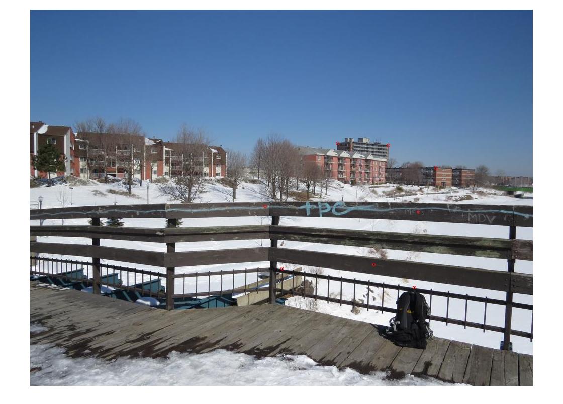
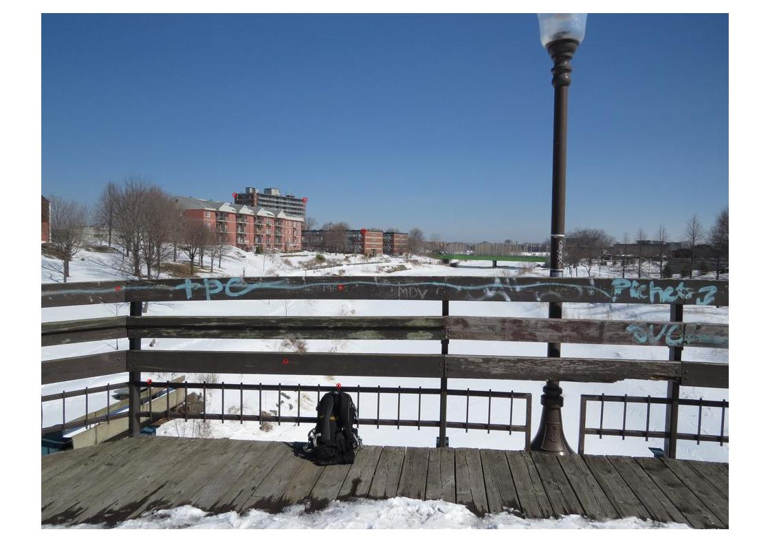
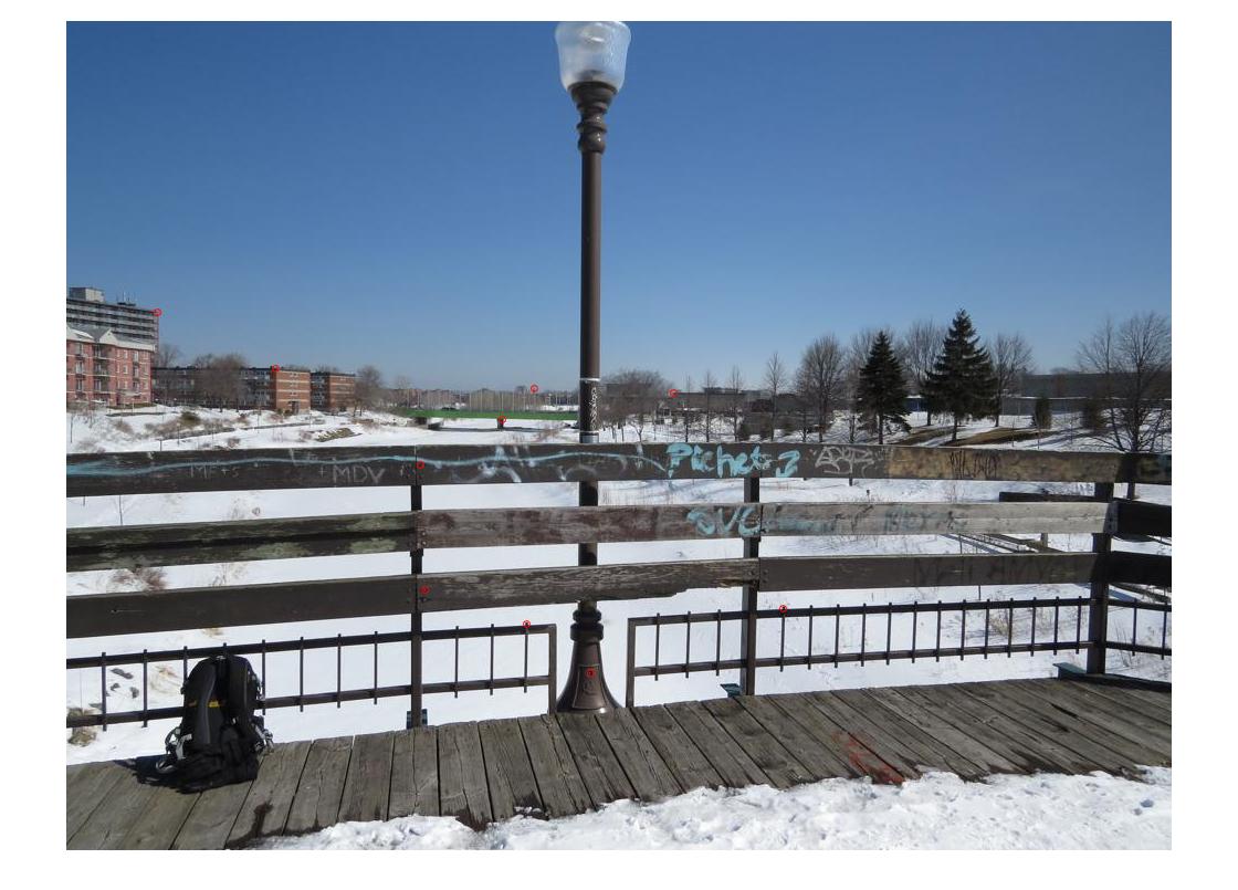
From the given set of images, an image in the middle of the scene was determined as reference image and
the other images were warped into its geometry, i.e. the other images are projected onto the image plane of
the centre image. For all other images, a respective homography was
calculated and applied using the function from Warmup.
Finally, the images have to be blended in order to get the panorama mosaic. To do this, I selected
a correspondence point from two images which should be blended. Based on this correspondence (in
coordinate system of the reference image), I calculated the required space of the new canvas in every direction.
Subsequently, I filled the new defined canvas with the warped images where again the correspondence point
served as orientation point.
Results
Feature matching As the features were selected and matched manually, no further correction or evaluation steps were requires.
Following features have been extracted:
| image 1, series 1 | image 2, series 1, matches to image 1 | image 2, series 1, matches to image 3 | image 3, series 1 |
| 
| 
| 
|
| image 1, series 2 | image 2, series 2, matches to image 1 | image 2, series 2, matches to image 3 | image 3, series 2 |
| 
| 
| 
|
| image 1, series 3 | image 2, series 3, matches to image 1 | image 2, series 3, matches to image 3 | image 3, series 3 |
| 
| 
| 
|
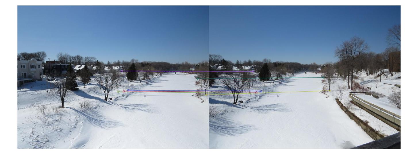
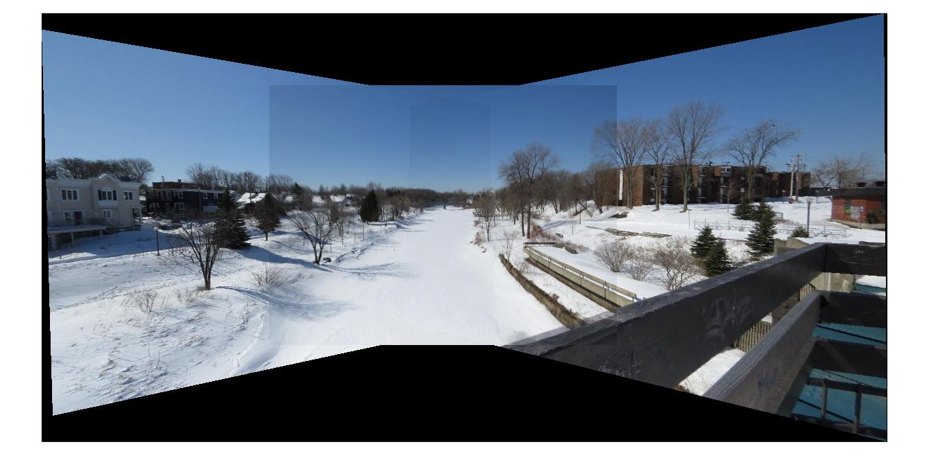
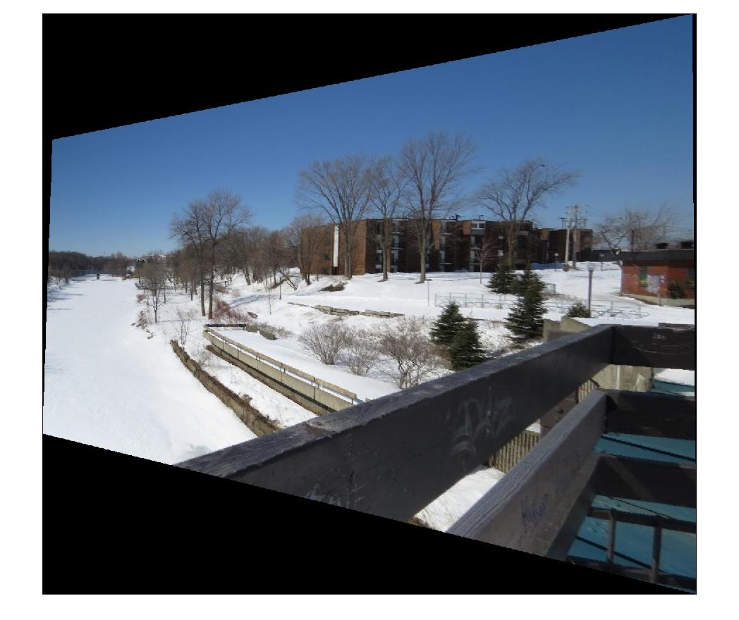
Image warping and image blending Series 1:
| left homography | blended panorama | right homography |
| 
| 
|
| left homography | right homography |
| 
|
| left homography | blended panorama | right homography |
| 
| 
|
| left homography | blended panorama | right homography |
| 
| 
|
Discussion
As visible, computation of homographies worked well, showing only minor deviations between
the contours at the overlapping regions of two images. An example of such a deviations is visible
at the wall in series 2 where the left image overlaps the right image.
Apart from that, the algorithm works well and image blending is correct. Only, small
differences in colors have not been corrected what makes visible the boarders of the original
images.
Part 2: Automatic matching
Methods Automatic matching requires less user interaction, however, the process is more complicate and consists of following steps:
1. Feature detection
1a. Adaptive Non-Maximum Suppression
2. Extraction of feature descriptors
3. Feature matching
4. Homography computation using Ransac
5. Image warping
6. Image blending
Results and discussion
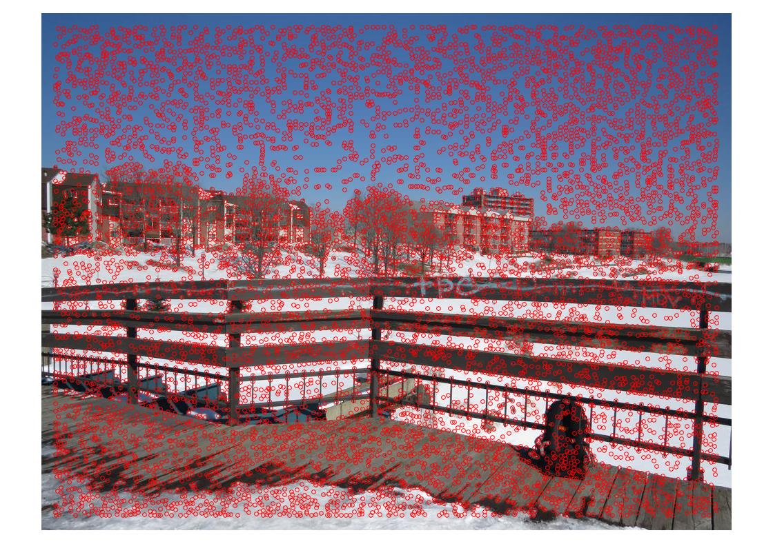
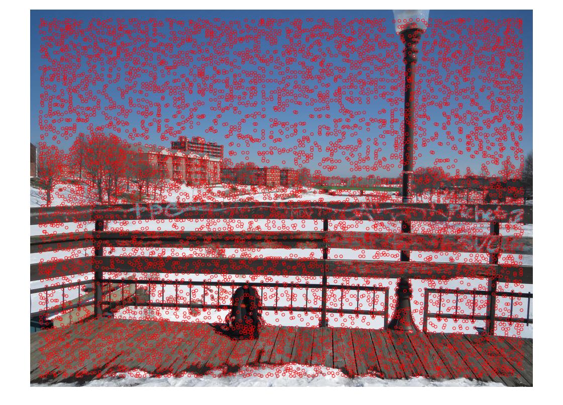
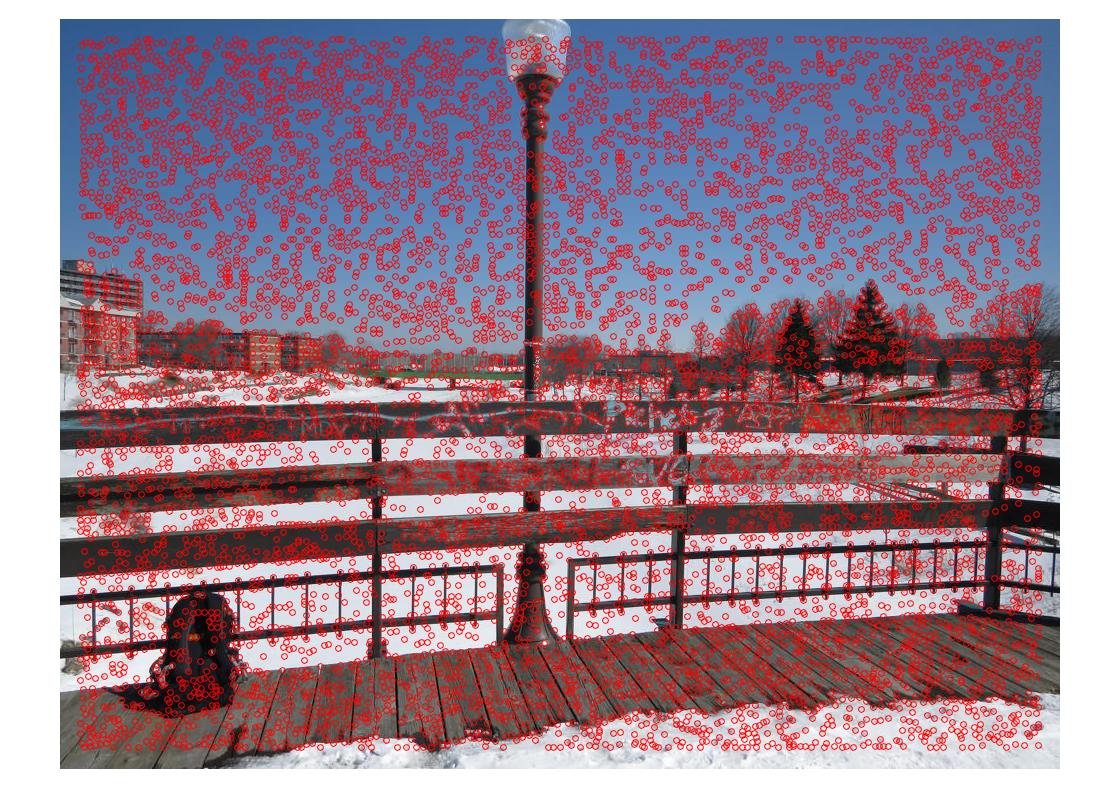
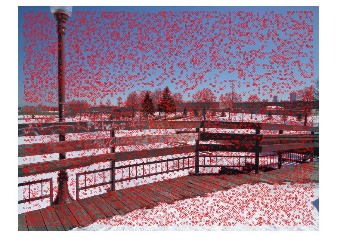
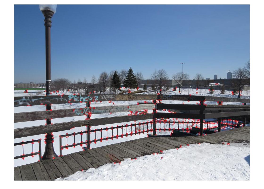
Feature detection Harris feature detection found more than 8000 features per image in series 2:
| Harris features img1 | Harris features img2 | Harris features img3 | Harris features img4 |
| 
| 
| 
|
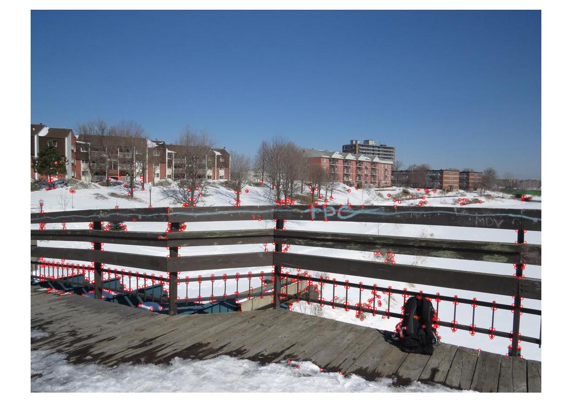
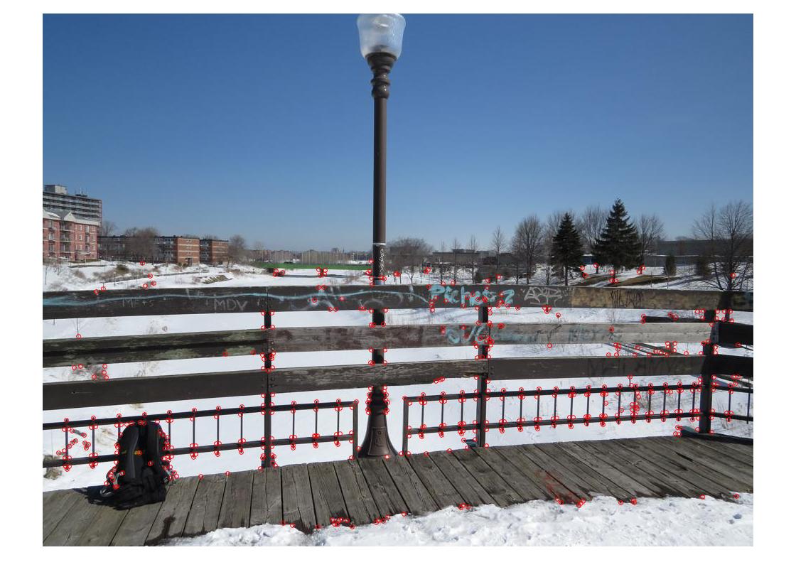
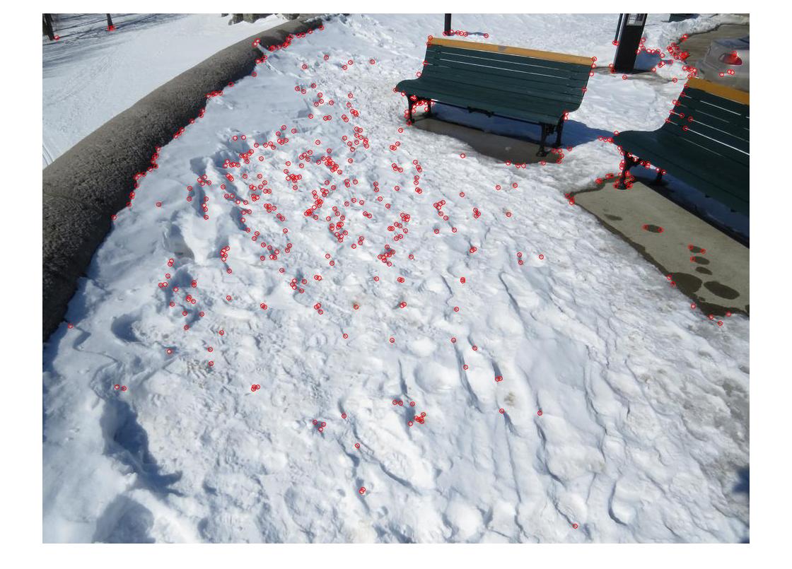
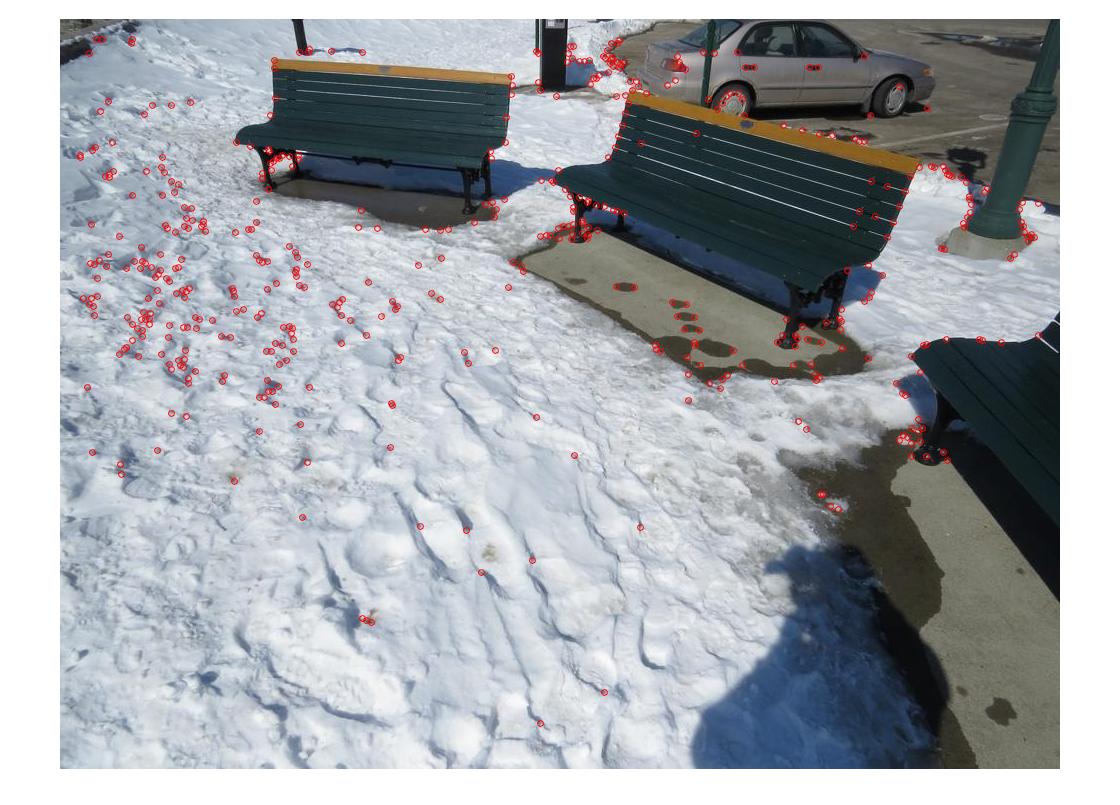
Adaptive non-maximum suppression Applying the adaptive non-maximum suppression retains the 500 most descriptive features. These features now are located at spots in the image with very distinct textures. This is evident when compared to the results from above from series 2:
| Harris features img1 | Harris features img2 | Harris features img3 | Harris features img4 |
| 
| 
| 
|
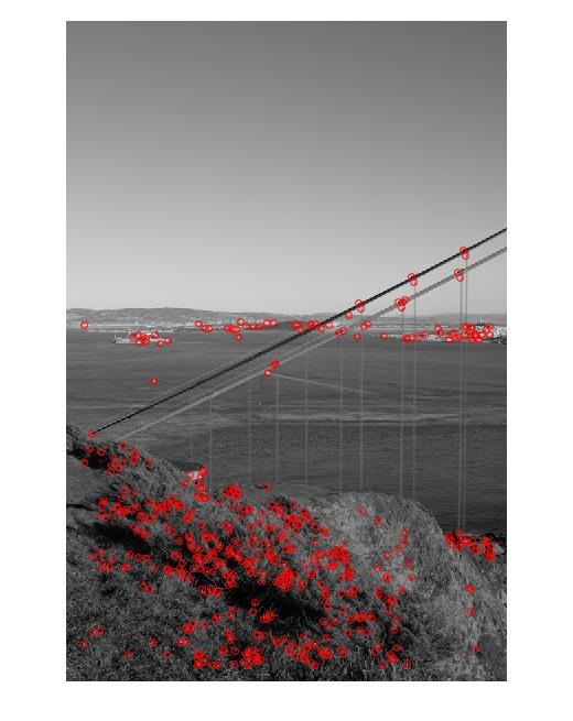
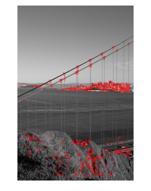
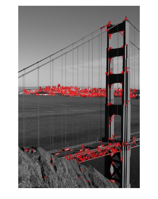
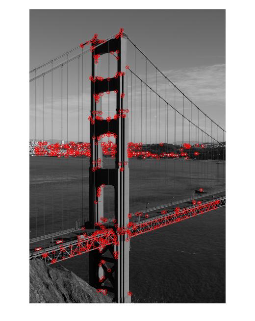
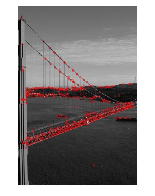
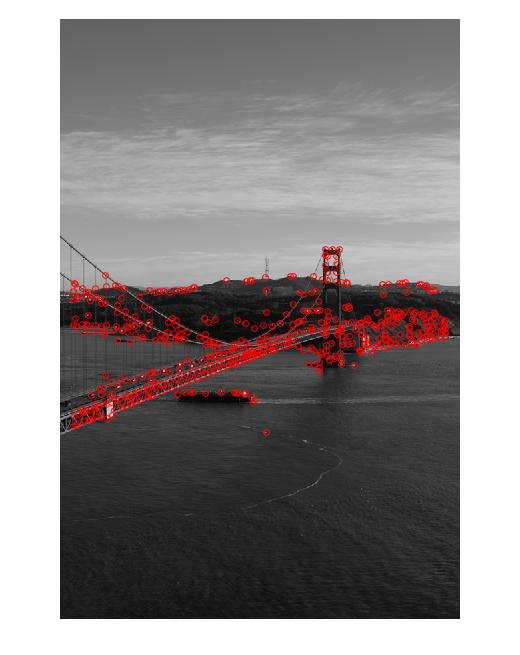
For the Golden Gate Bridge, following features were retained:
| Harris features img1 | Harris features img2 | Harris features img3 | Harris features img4 | Harris features img5 | Harris features img6 |
| 
| 
| 
| 
| 
|
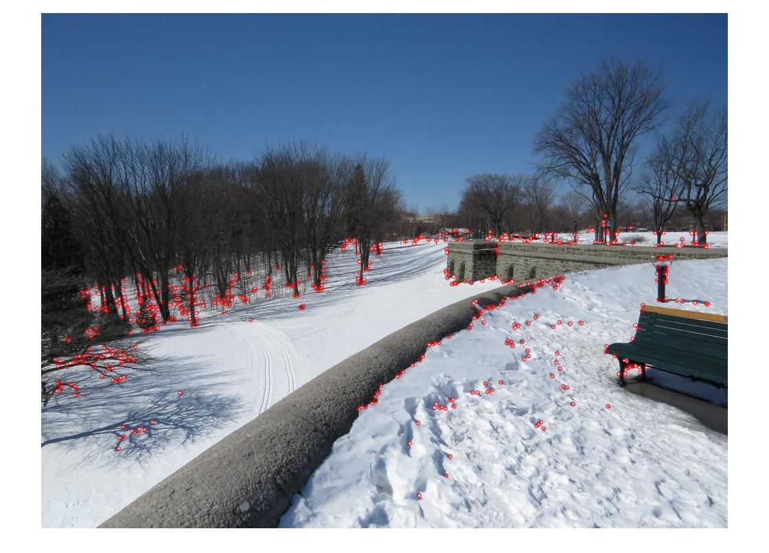
For the third data set, the features after suppression are the following:

| 
| 
| 
|
| 
| 
| 
|
| 
| 
| 
|
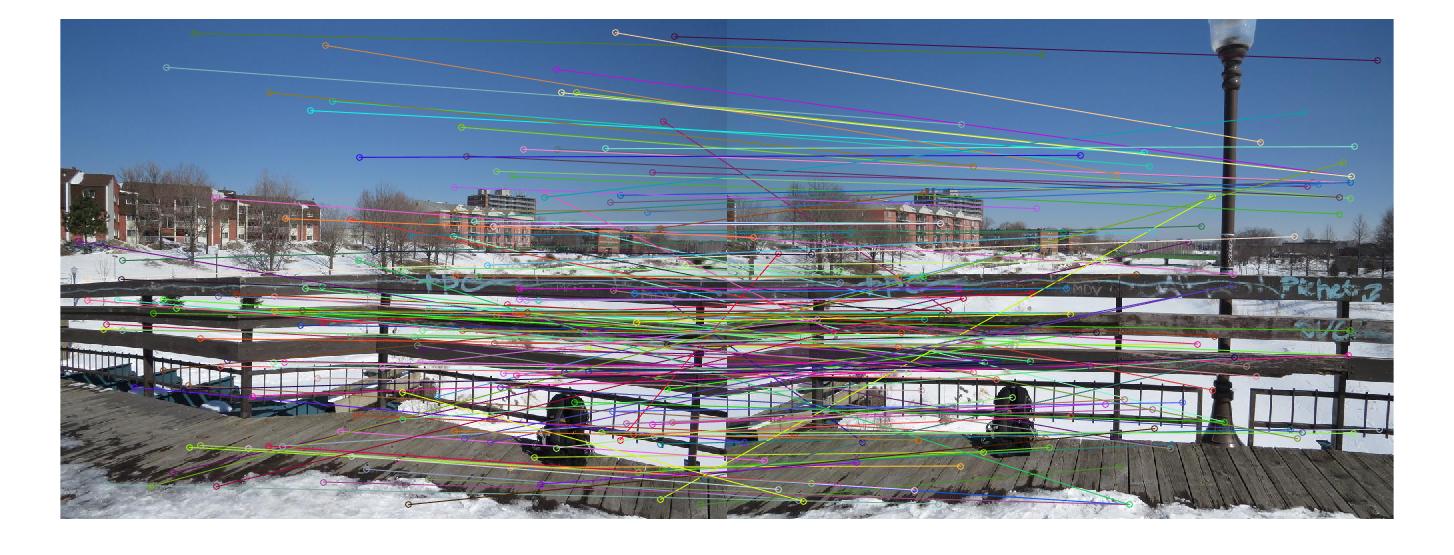
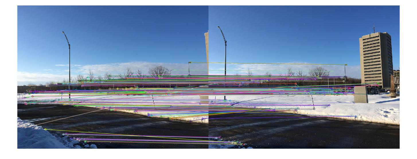
Feature matching The many features detected in regions with indistinct textures and, thus, small Harris scores have implications on the subsequent feature matching as it leads to many mismatches, i.e. features are detected as matching features, but obviously are not. The figure shows a set of matches where the initial features set was thinned out by i) filtering the features with very small Harris scores and by ii) picking a random set of 1000 features:
Feature matching in the suppressed features set, on the other hand, leads to more "real" matches:
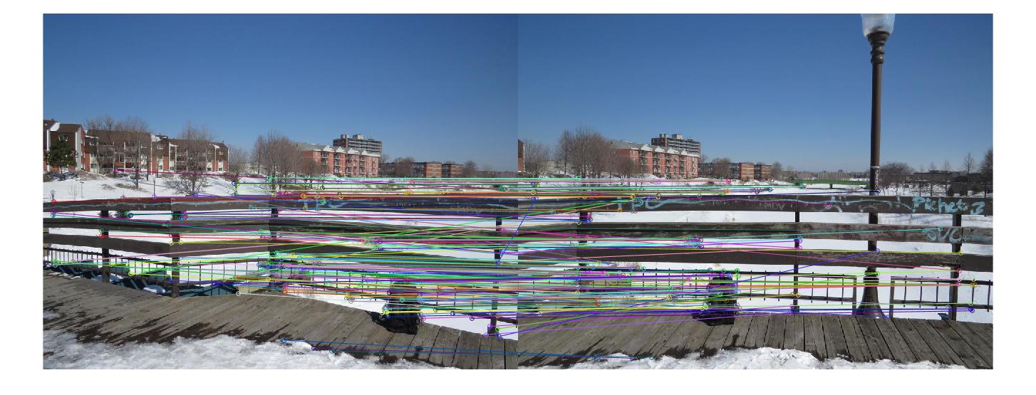
Another example from the Golden Gate Bridge:
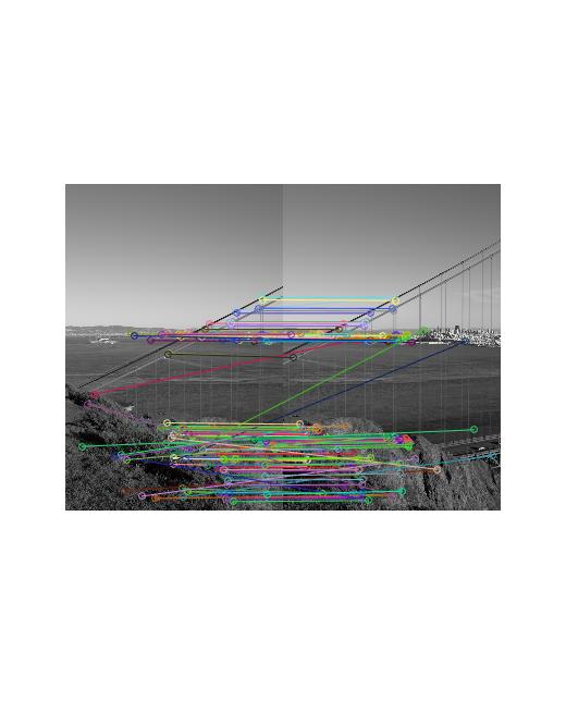
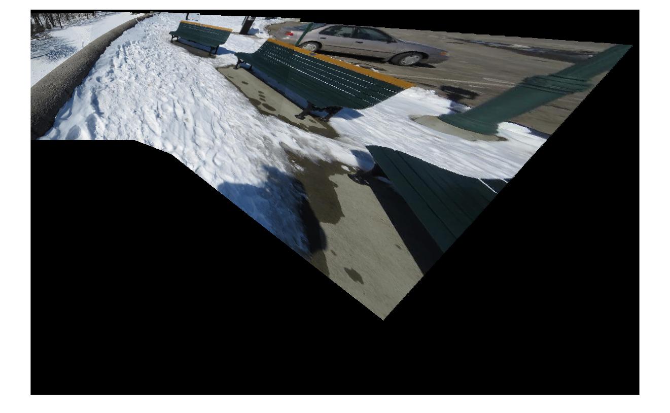
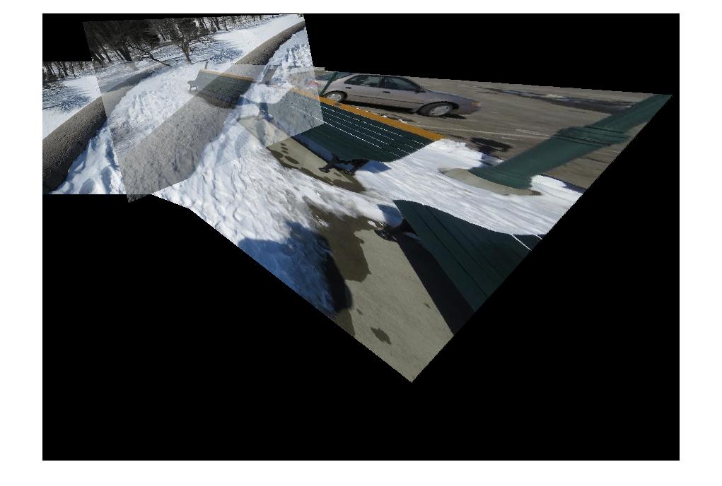
Warping and blending The final results look as follows:
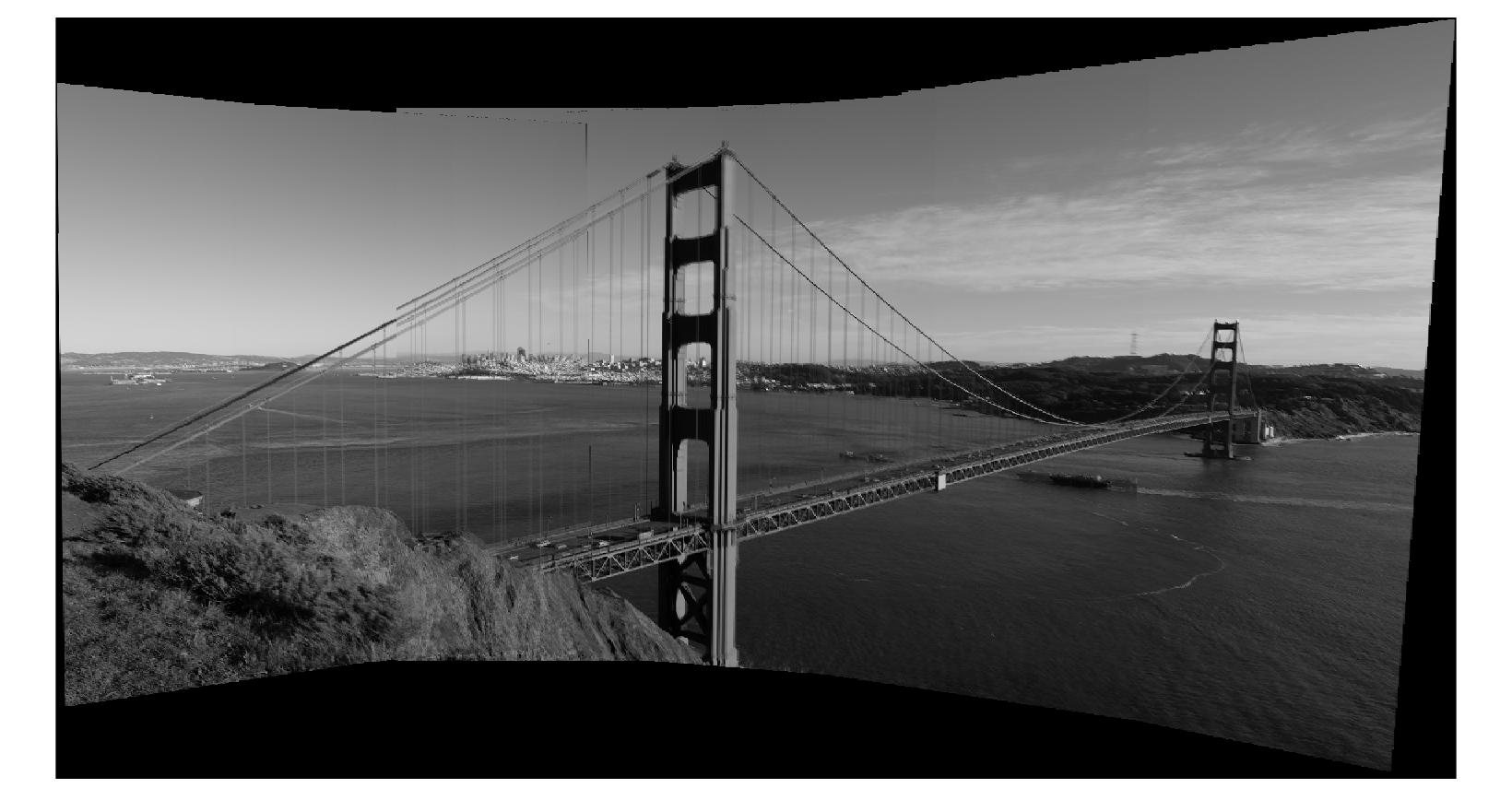
For the middle set of 4 images of series 3 (images 5 through 8), computation worked well, which is surprising, as many features in image 5 (left most) were detected within the bushes. Furthermore, the final panorama blending shows very large distortions as camera position between two images vary largely:
However, while for these series, the results are good in general with only minor artefacts where the
images overlap, the rest of the images in the third data set did not work very well .
For the first four images, the left most image was not transformed and placed correctly:
This is surprising as the detected and retained features looked good, showing many
obvious matches to the image on the right (see above).
For the last 4 images, only a set of 3 images was warped and blended correctly while the process for the fourth image
failed:
and for the last 4:
This is surprising as the threshold in Ransac to delineate inliers from outliers was reduced to 0.8 instead of 1.2.
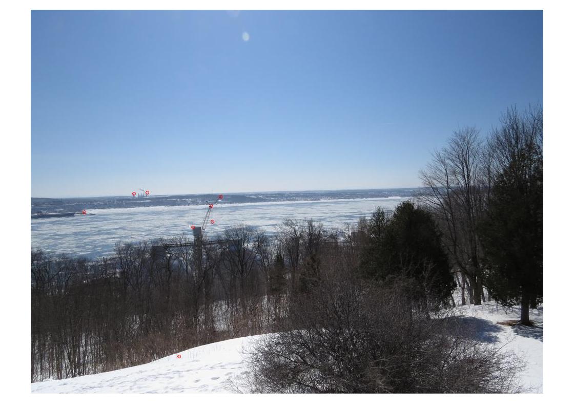
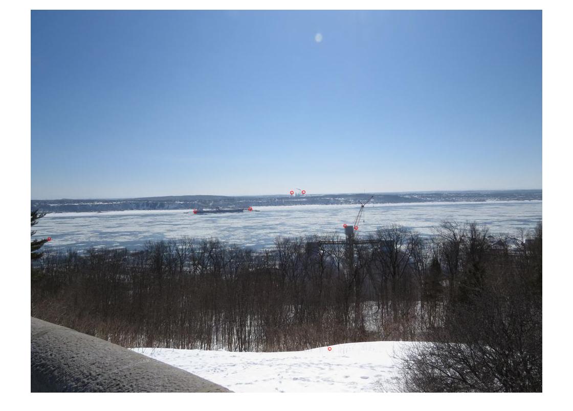
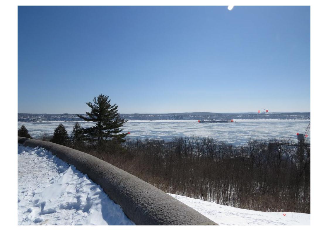
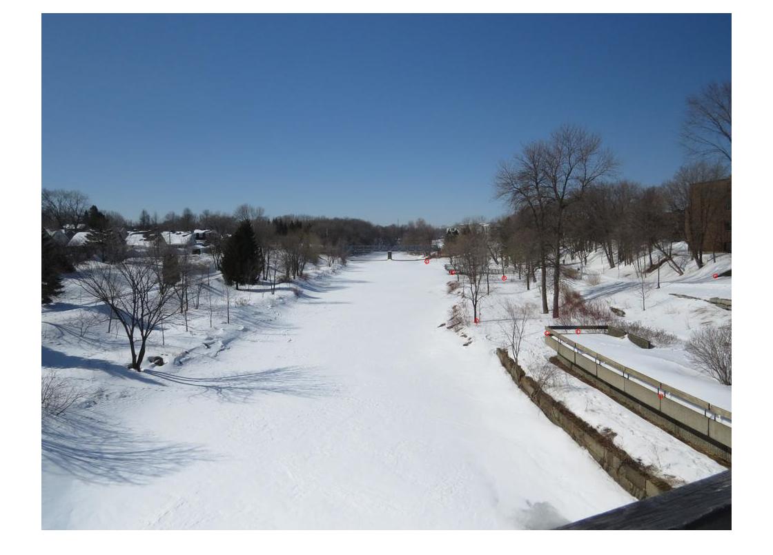
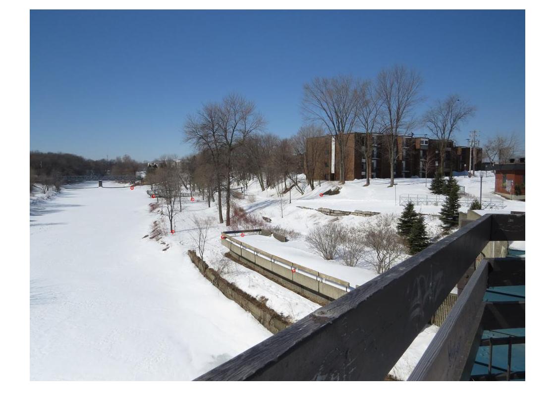
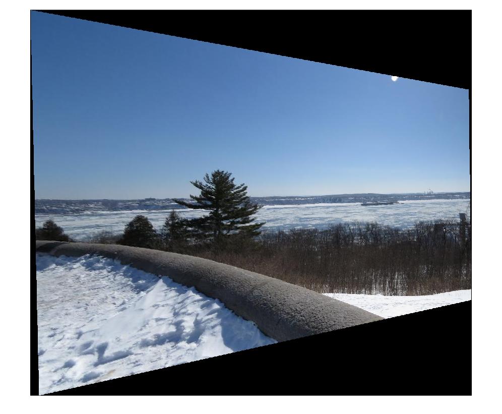
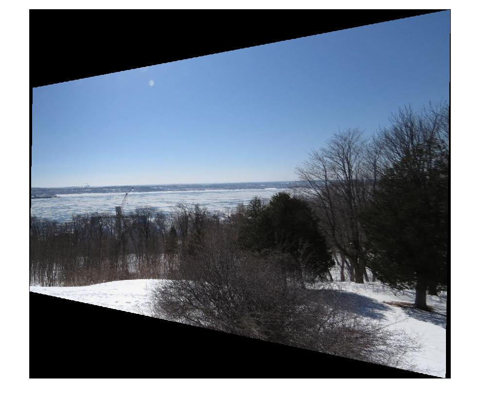
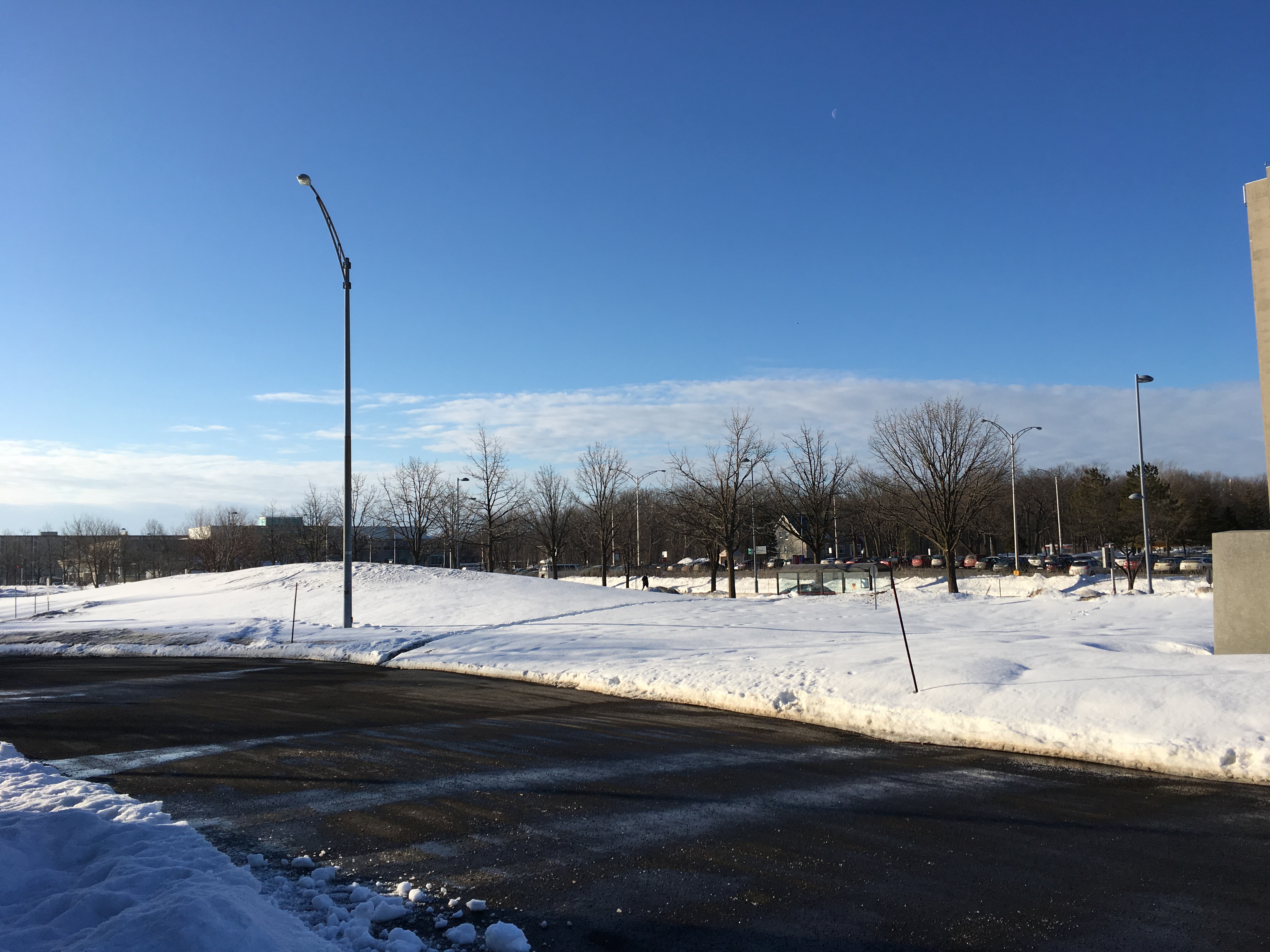
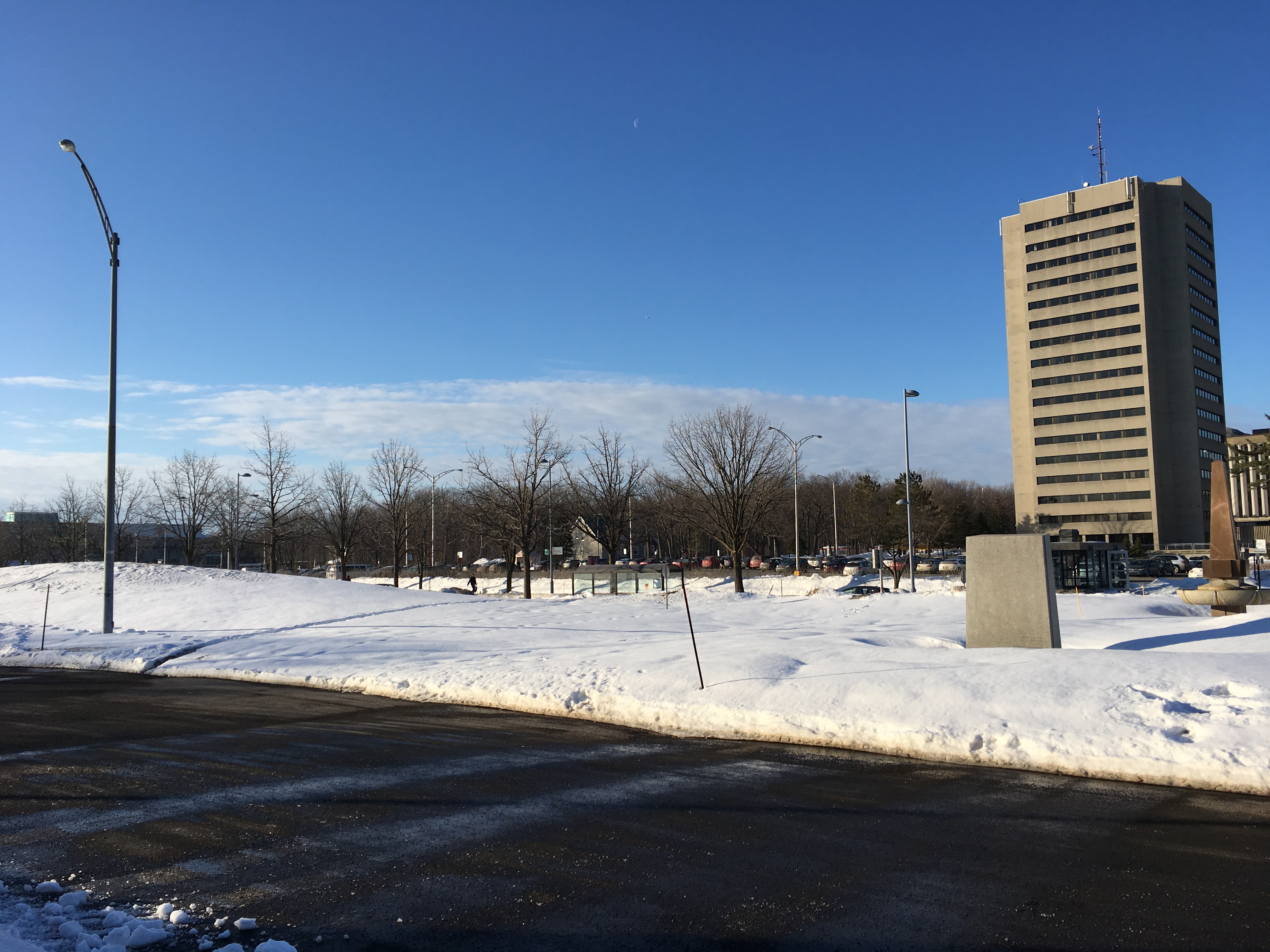
Part 3: Own images In this section, the same pipeline as described in Part 2 was used for computation of panoramas.
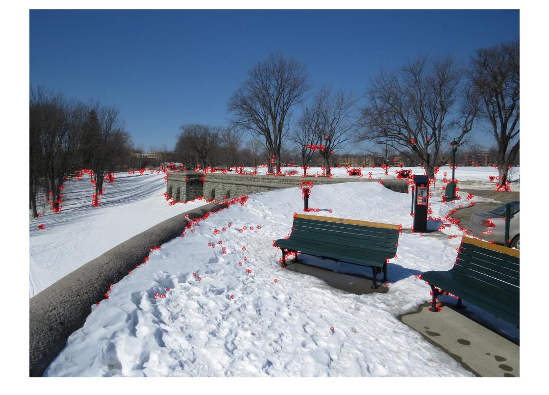
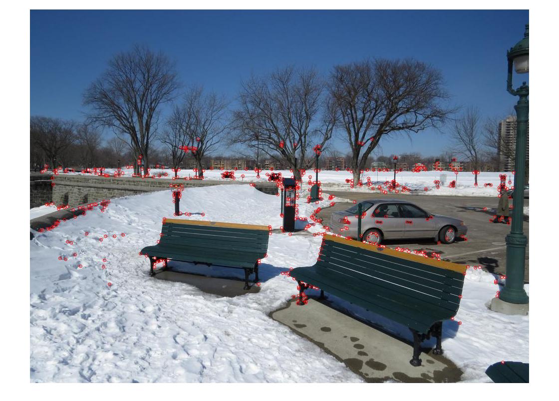
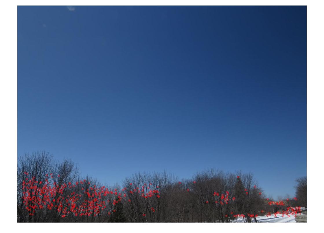
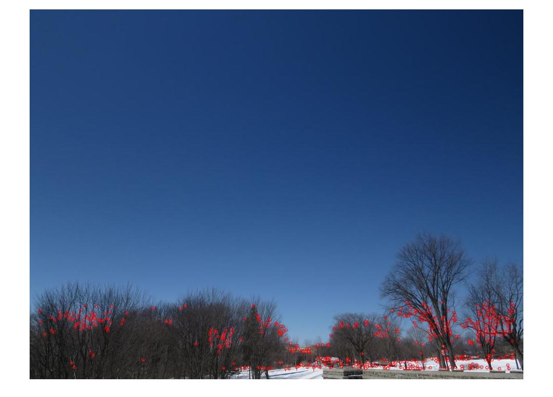
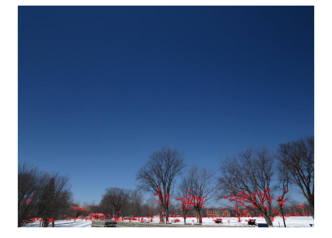
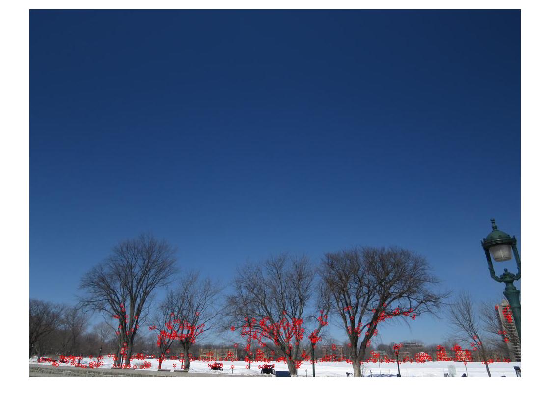
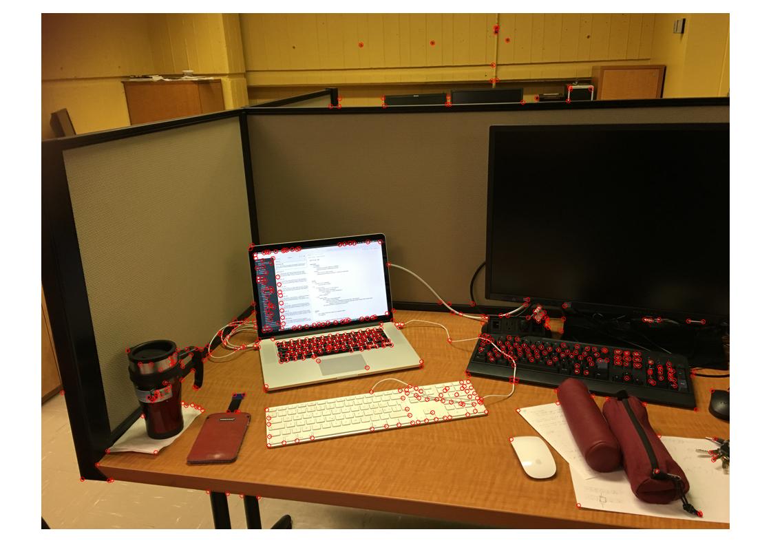
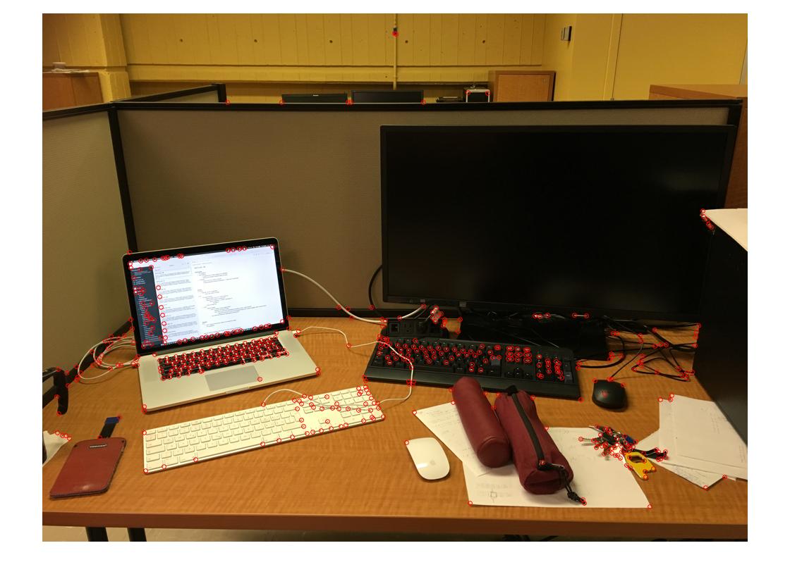
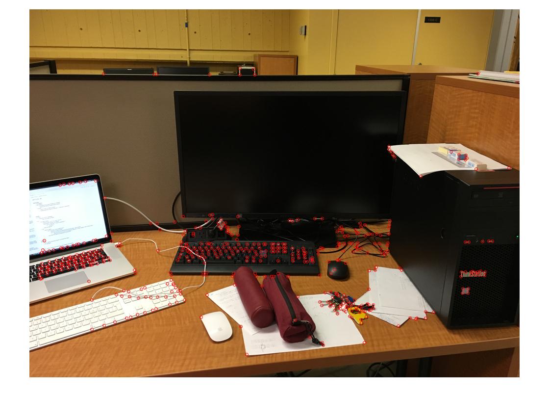
Results and discussion Features (second image row) for the first set (top row) after non-maximum suppression are the following for the three pictures:
| left image | centre image | right image |
| 
| 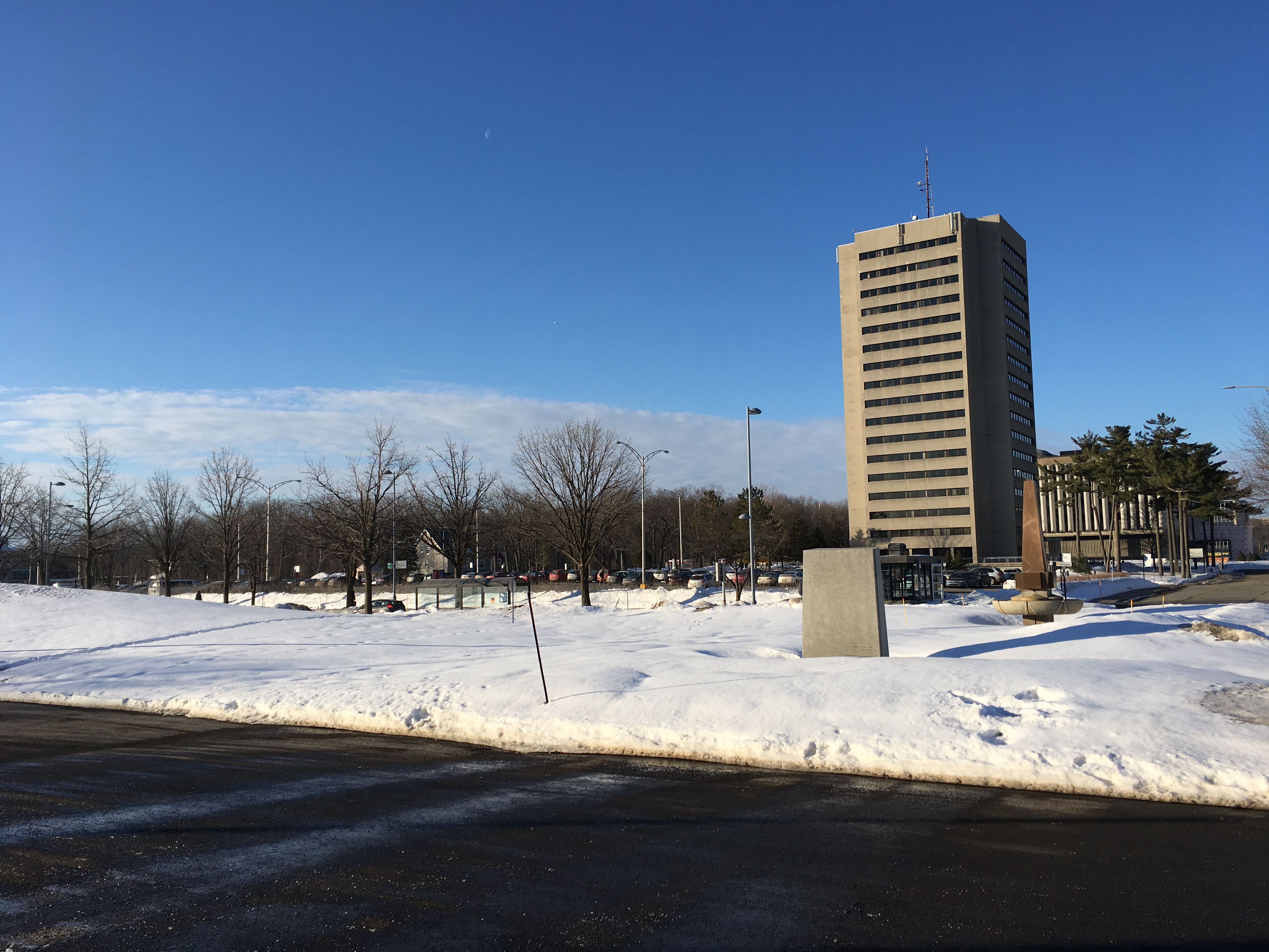
|
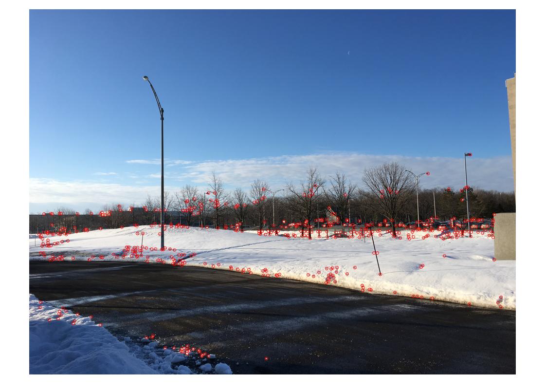
| 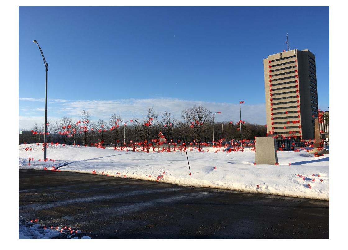
| 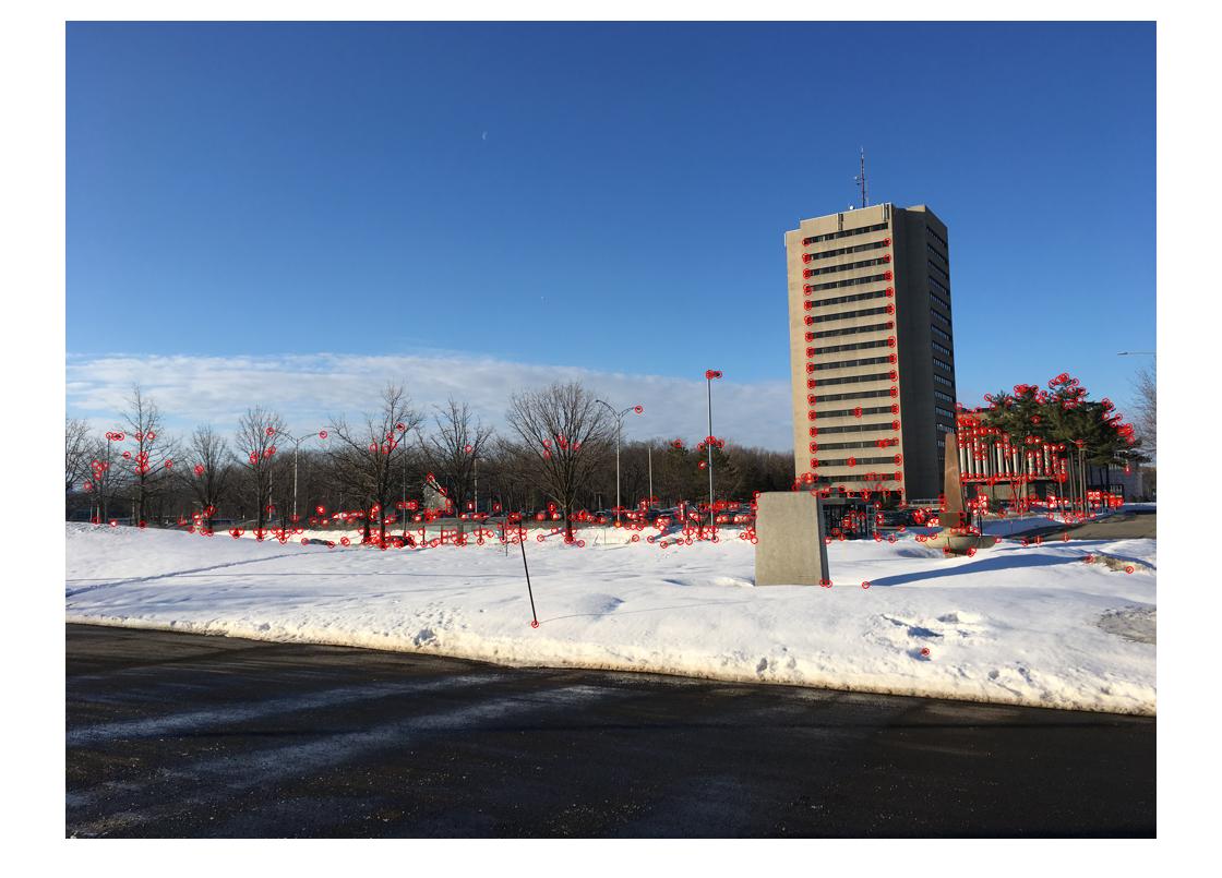
|
From a first view, only a small number of mismatches is contained.
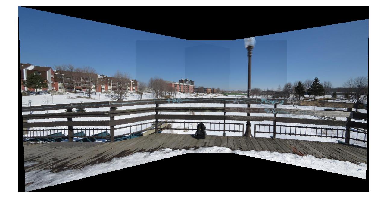
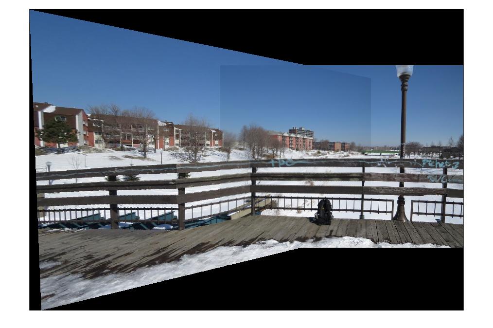
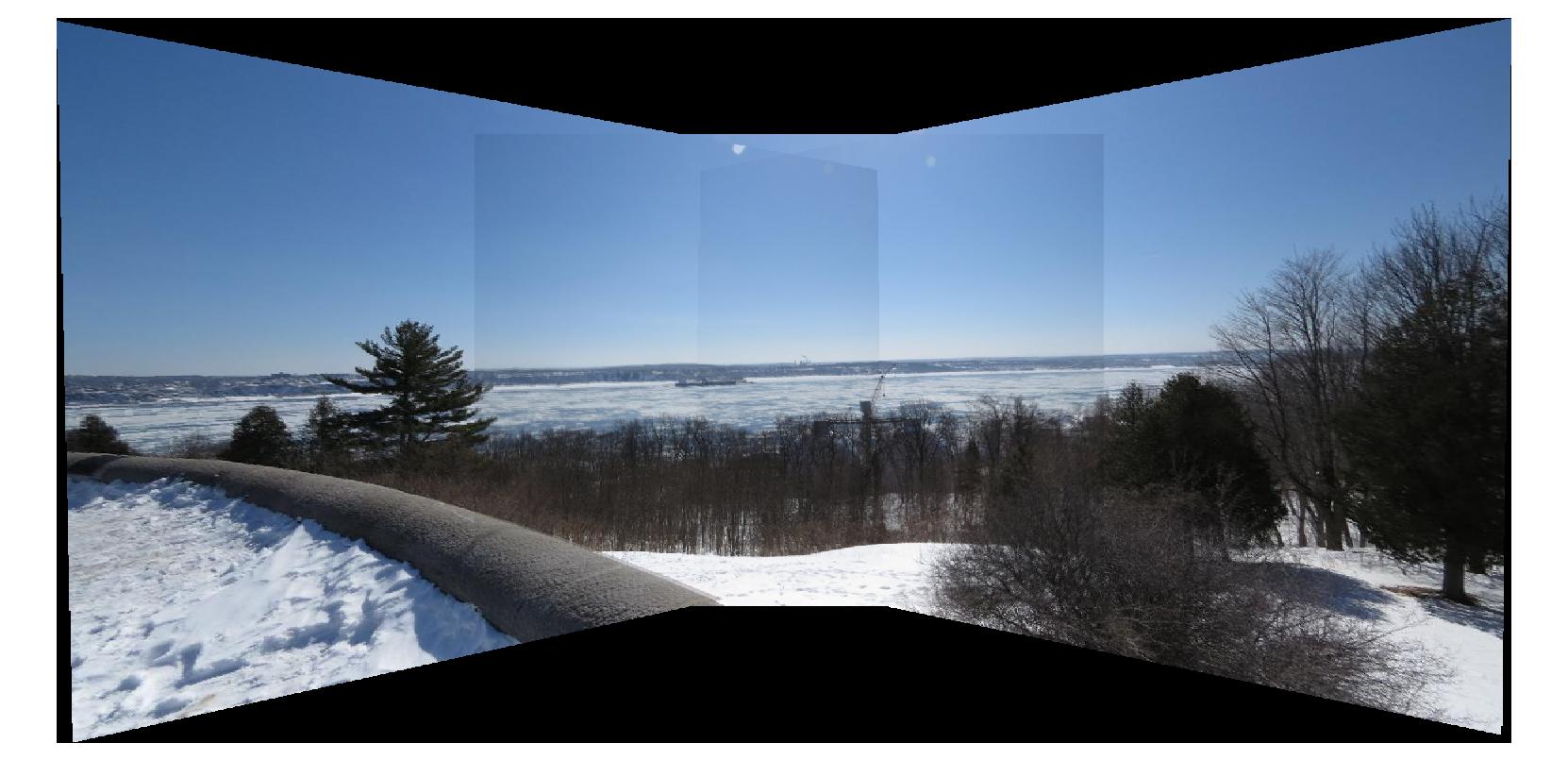
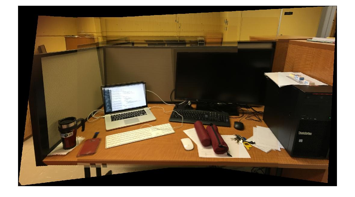
Calculation of homographies and blending results in this panorama:
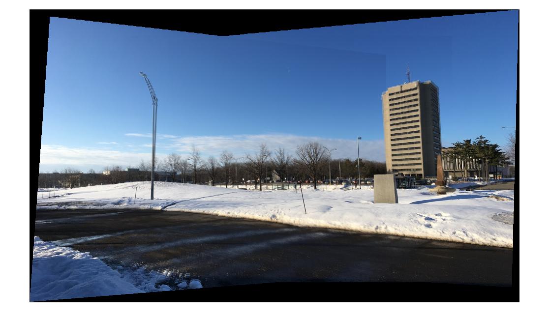
As visible, the images do not match perfectly but show some slight artefacts (blurred contours)
where objects in multiple images overlap. I ascribe this to the image acquisition geometry rather
than to algorithm as homography computation for the depicted set with many good matches should
work very well.
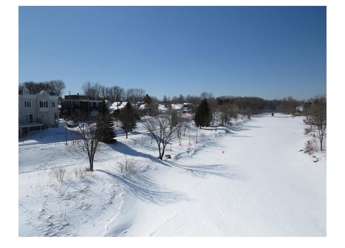
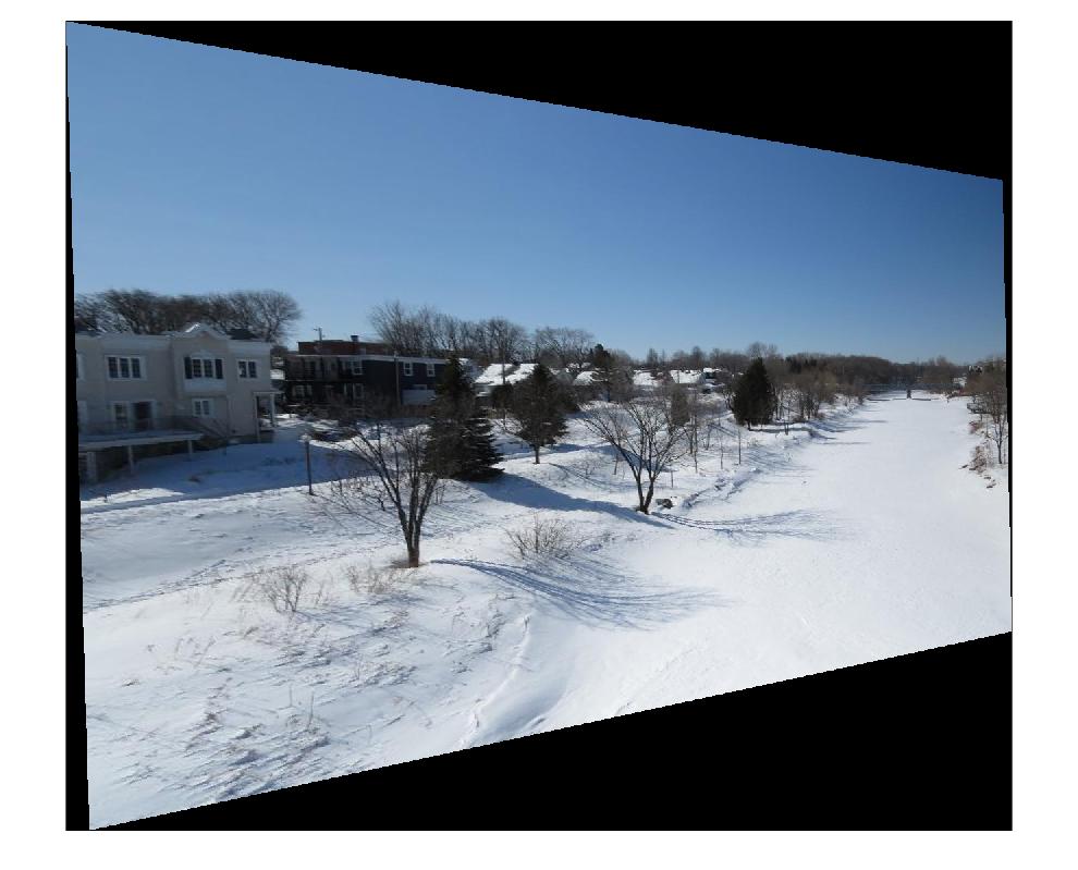
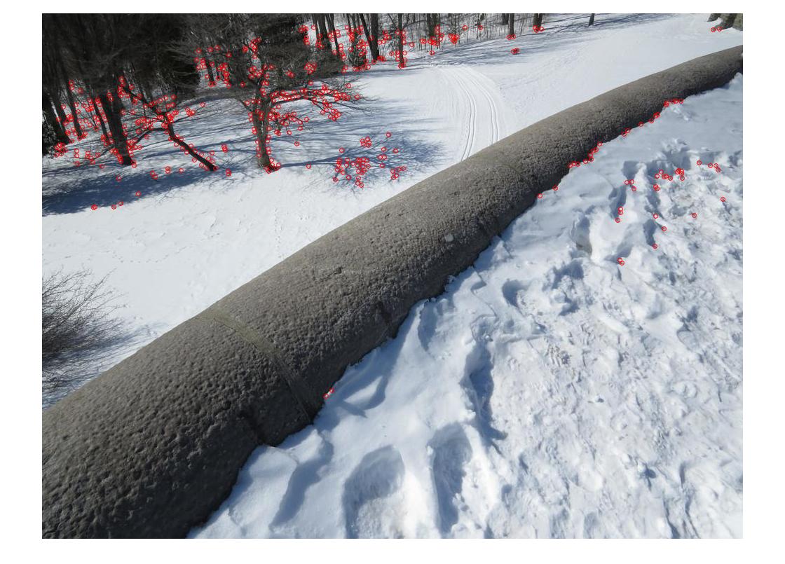
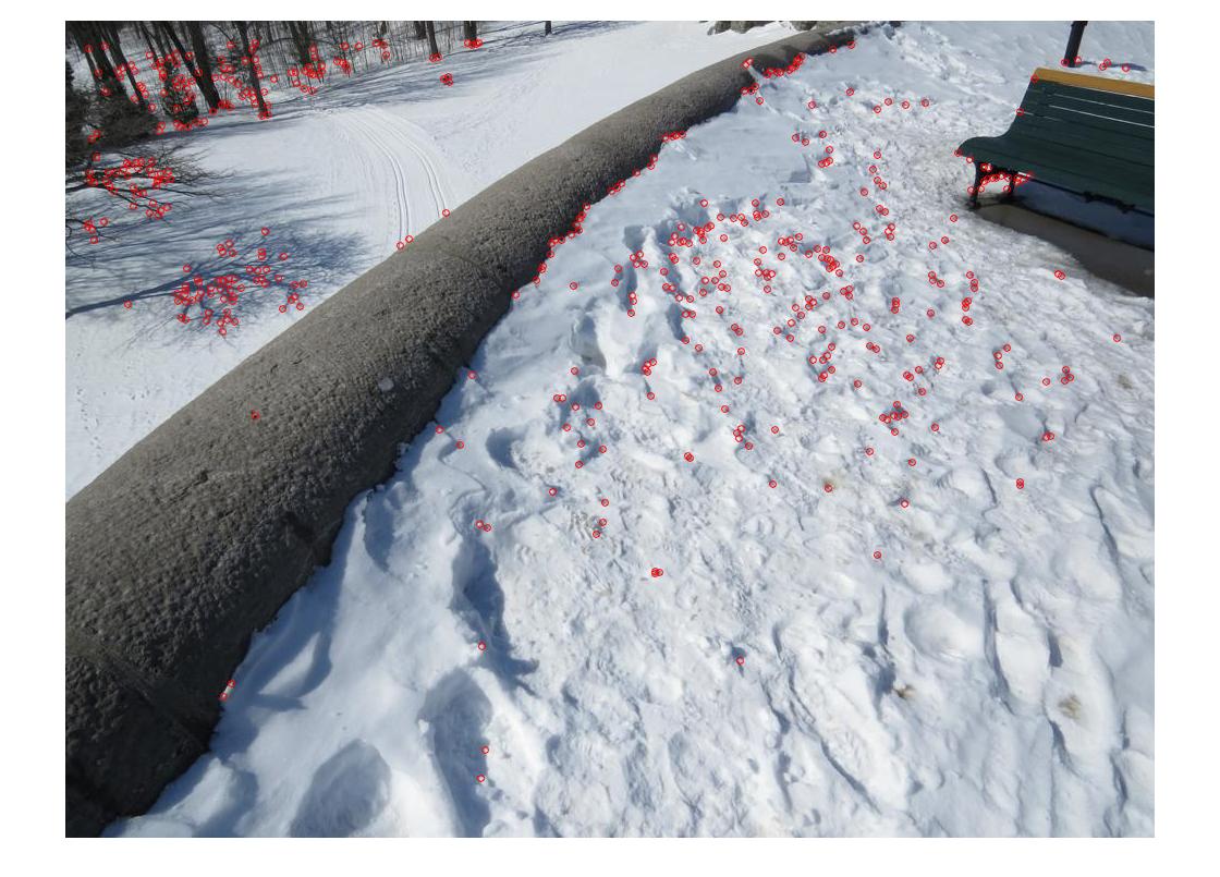
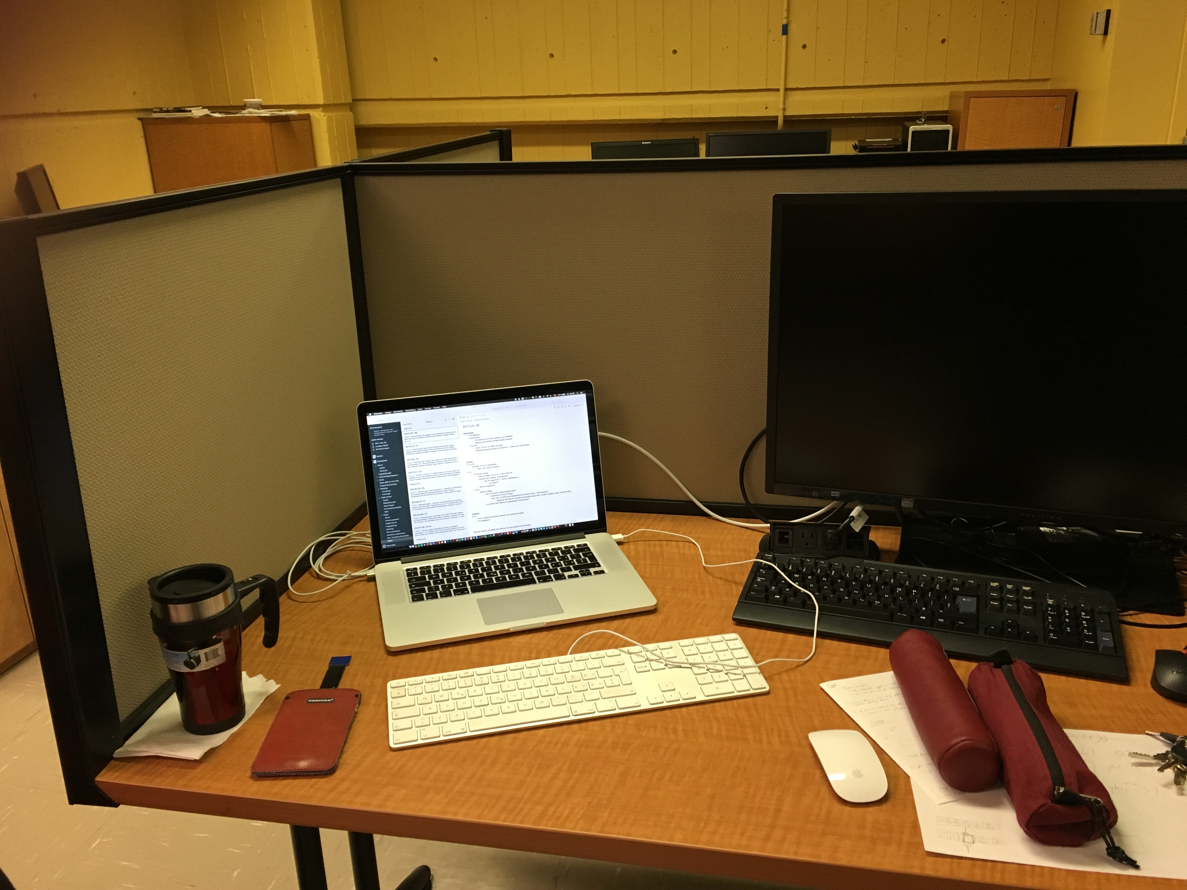
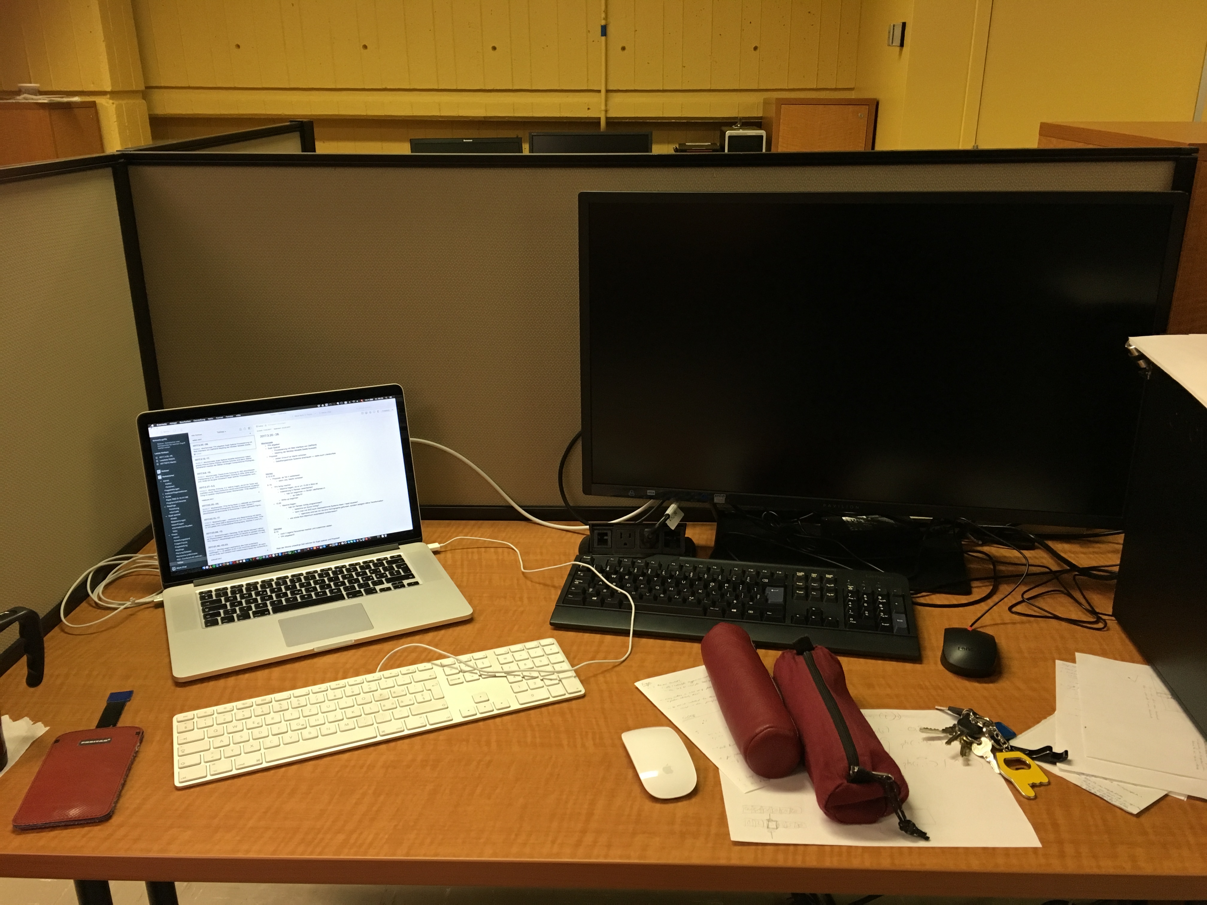
The same problem is even worse in set 2. I used these images:
| left image | centre image | right image |
| 
| 
|
where following features were detected and retained:
| left image | centre image | right image |
| 
| 
|
For the left-centre image pair, the matches are:
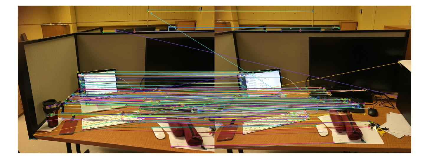
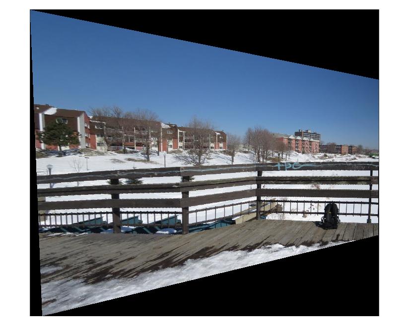
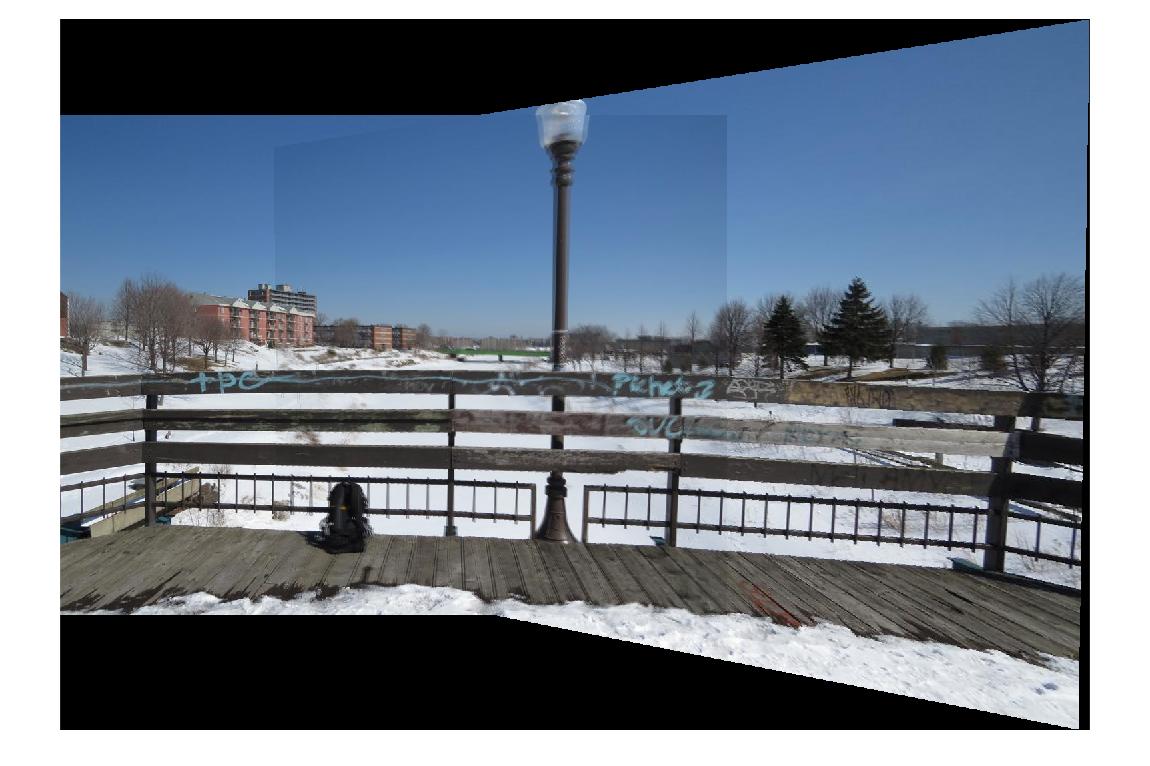
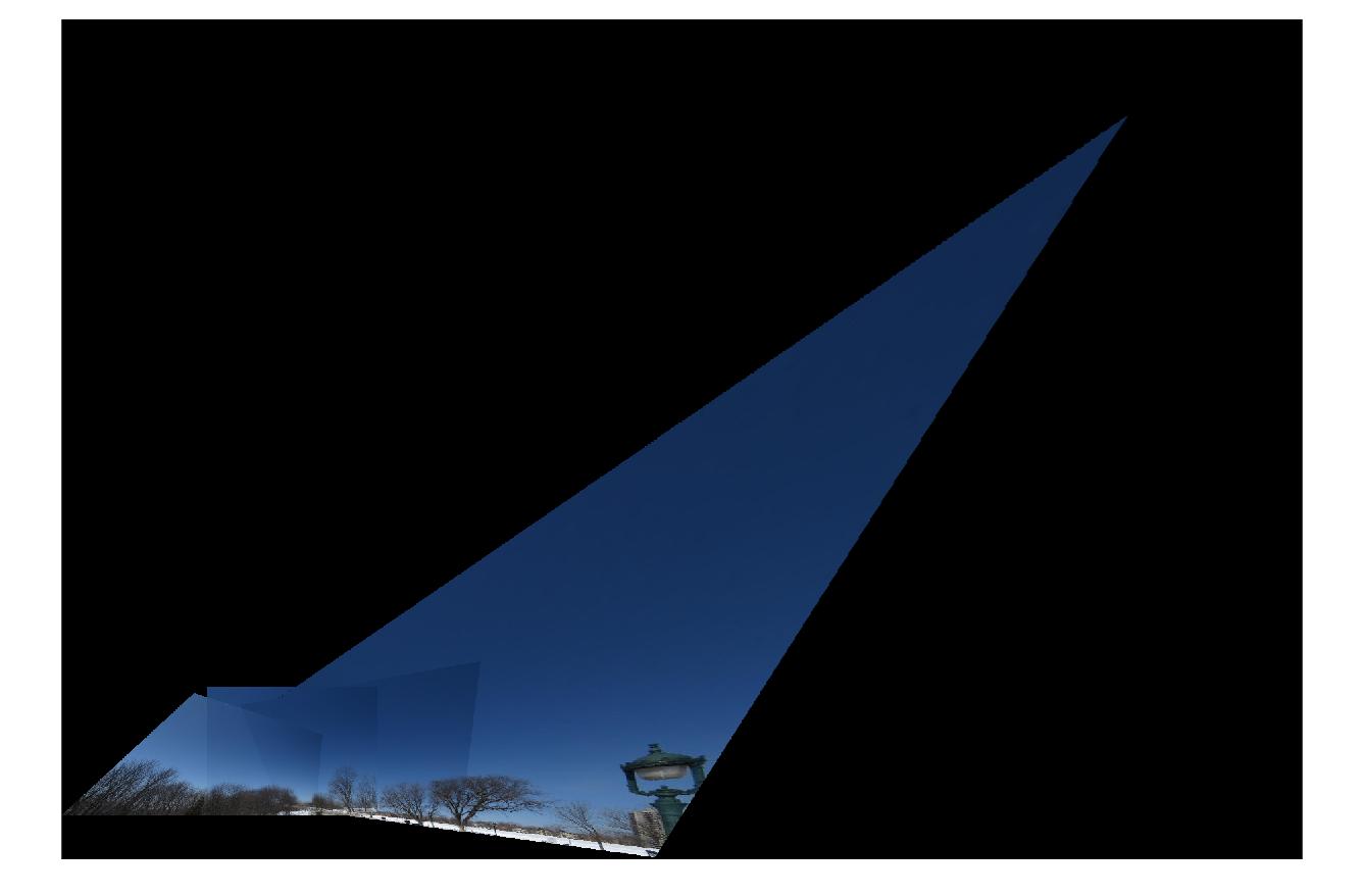
Again, there are not many obvious mismatches. However, the final results after homography computation, image warping and blending is not very good:
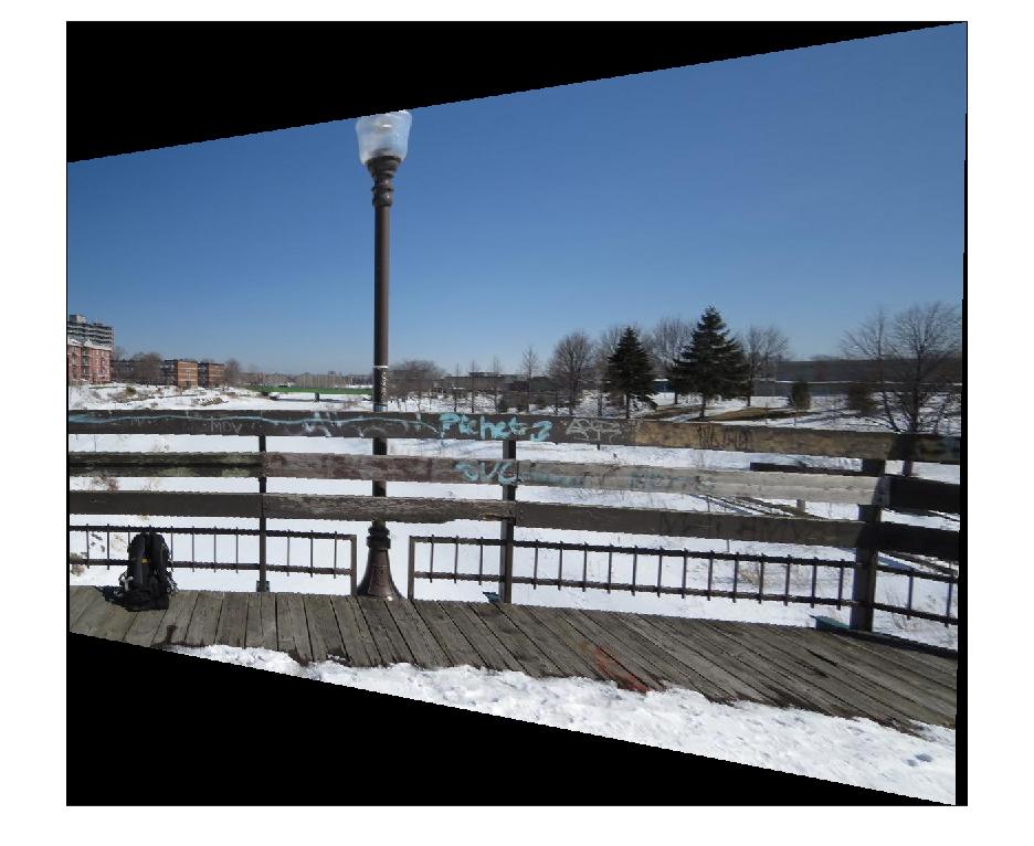
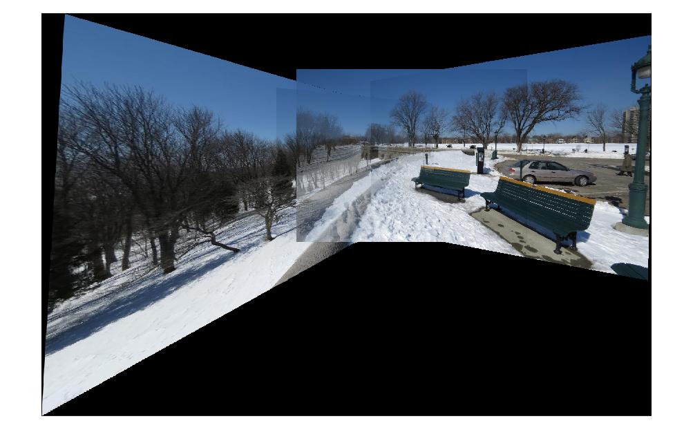
The panorama reveals some distinct discontinuities. On the other hand, blending of right and centre image only leads to a much better result:
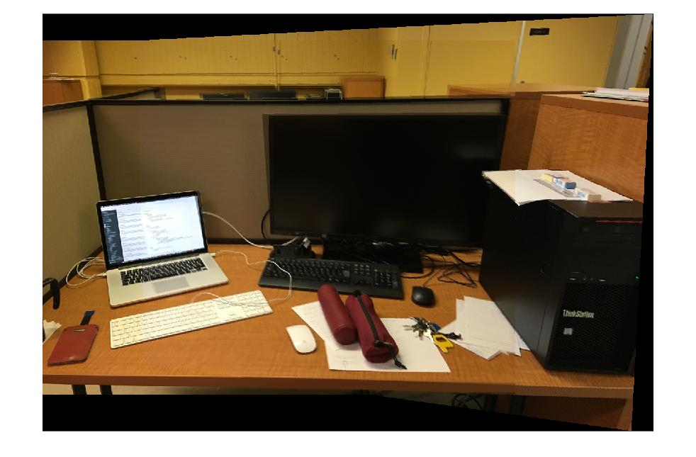
Thus, I expect that movement/rotation between acquisition of left and centre image was slightly too large what changed the projection centre. Therefore, the images can not be projected onto a common image plane (namely the plane of the centre image).