The goal of this assignment is to create a panorama from a set of photos. For that the following steps were implemented:
All these steps will be illustrated bellow together with the results.
"imgTrans = applyTransformation(img, H)", which would transform the image "img" by the homography matrix "H". In theory it suffices to apply H to all pixels positions of the image and then copying its intensities to their new position. In practice however such approach leads to three problems: (1) the final image will potentially have holes in places which were there was no correspondency from the original image, (2) there will be many pixels collapsing to the same location if the image needs to be warped (which is almost always the case) and (3) we do not know the size of the transformed image. To overcome problems (1) and (2) we can use the inverse of the matrix H and search on the original image for the pixels intensities for every point in the final image. And to overcome problem (3) we can apply H to the extremes point locations of the original image and from there take the minimum and maximum values to know the final size of the image. The result can be seen bellow.
Target image.
Image after applying the transformation.
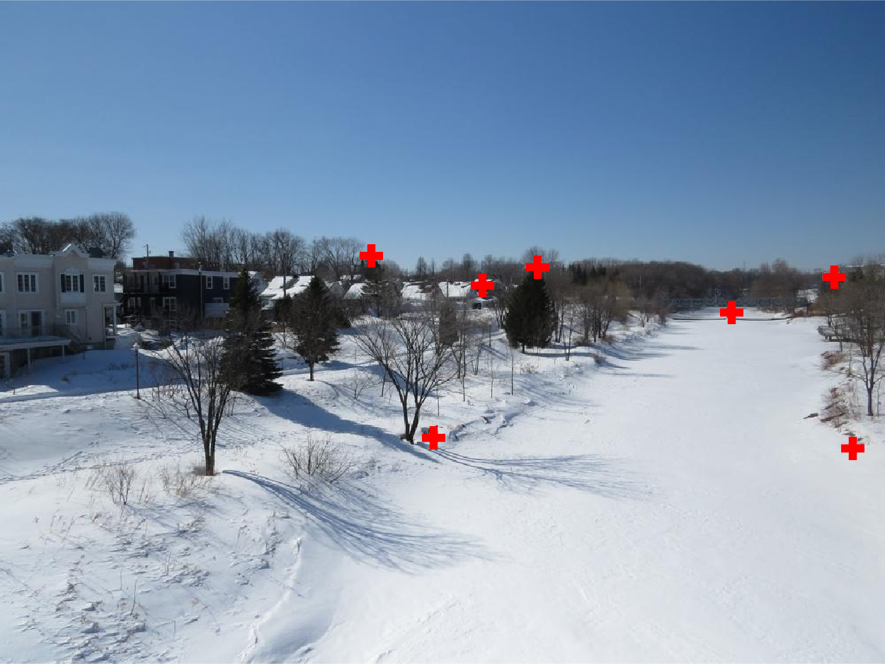
Image 1 with points related to image 2.
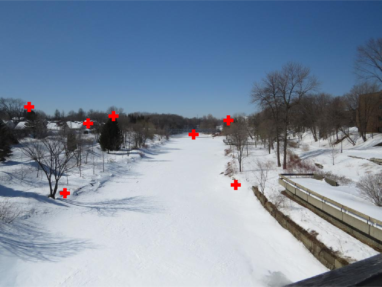
Image 2 with points related to image 1.
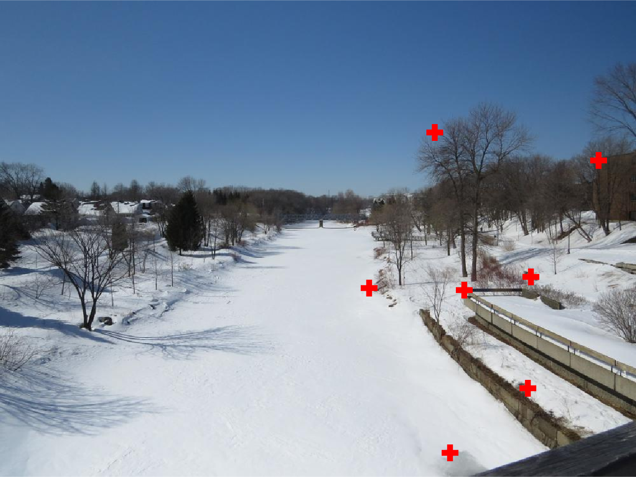
Image 2 with points related to image 3.
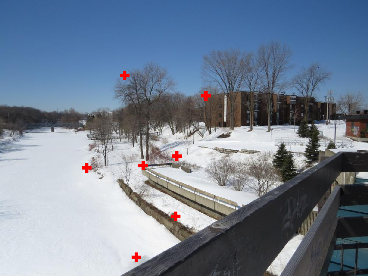
Image 3 with points related to image 2.
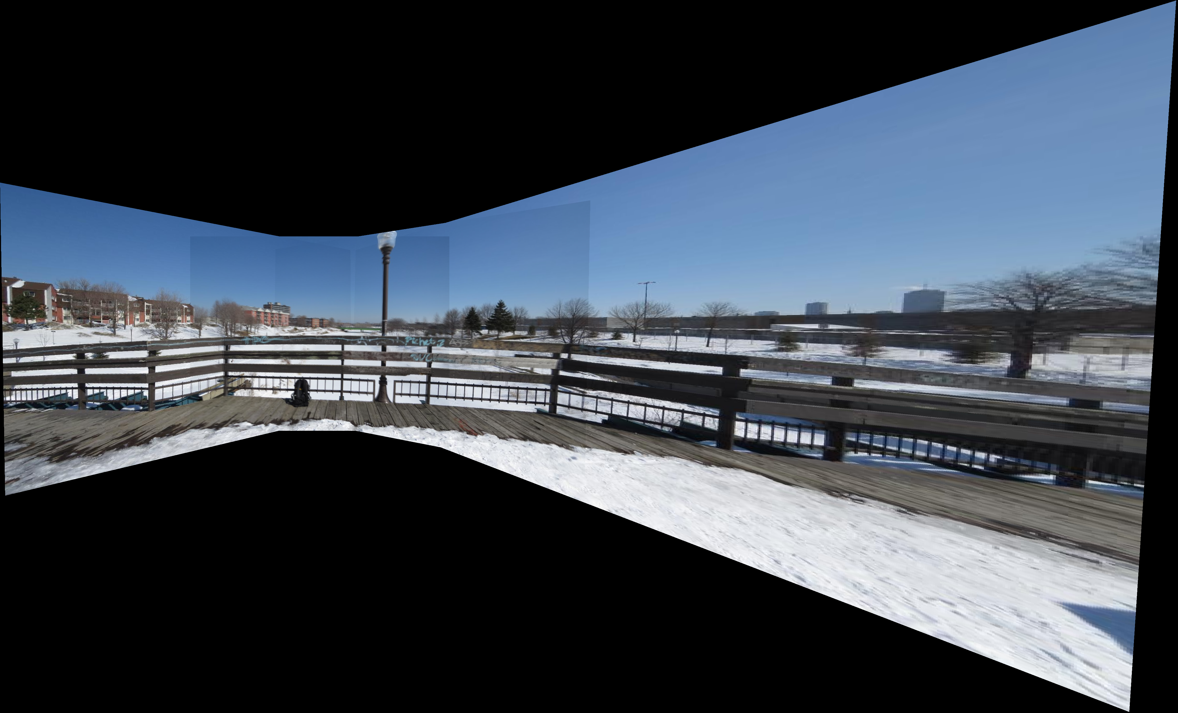
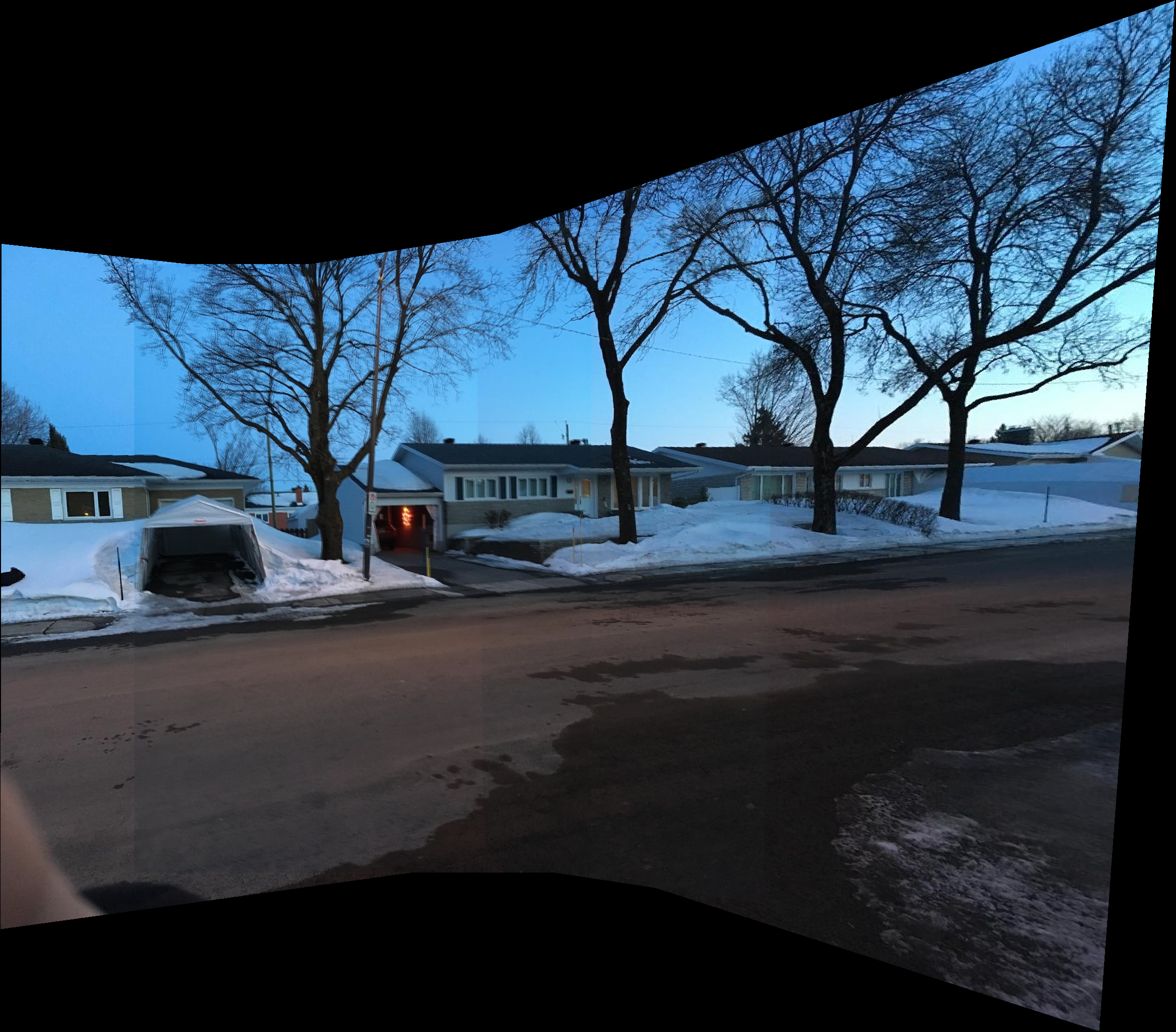
The result is an interpolation of all images in their right place. This "right place" was for me the most difficult part of the assignment! I had a hard time trying to find a way to keep track of the image places while placing them in the final panorama. Finally my solution was to create a vector containing a translation for each image. As I deform a new image, I calculate its position and update all images that have been already deformed to reflect this new arrangement. In this result I also took the maximum intensity value from both images where they overlap. It was just an experiment to blend both images without visible artifacts in the sky and also to reduce the blur caused by misalignment.
Target image.
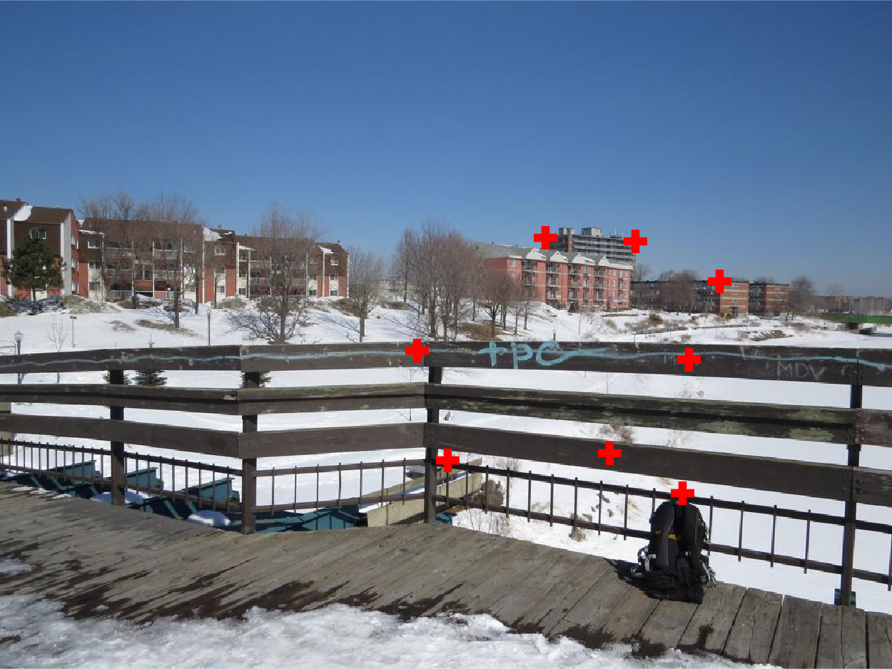
Image 1 with points related to image 2.
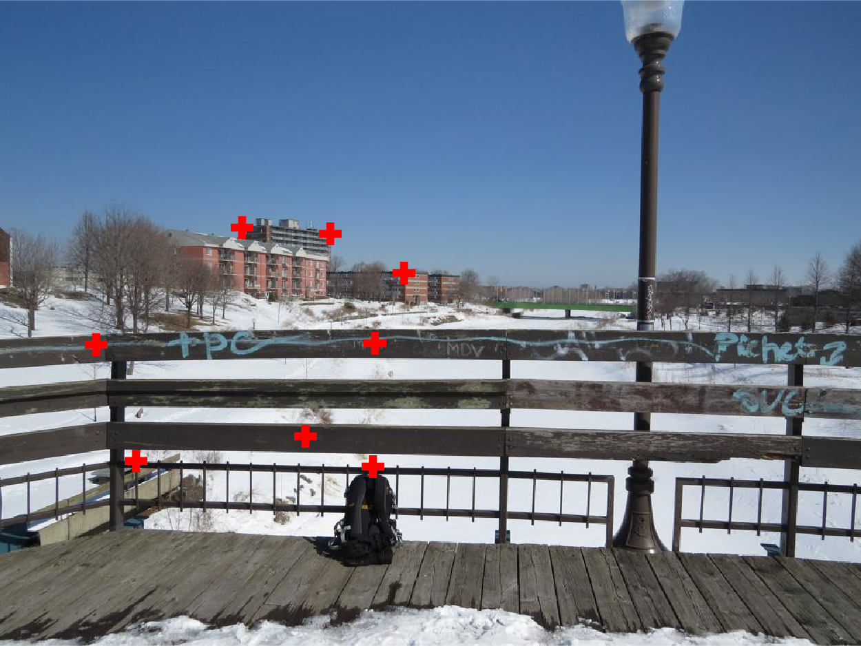
Image 2 with points related to image 1.
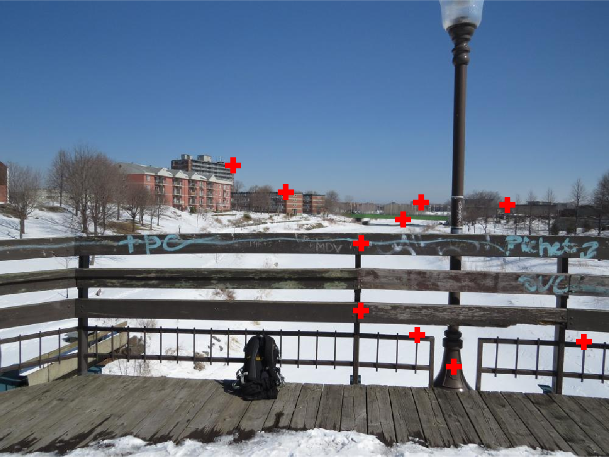
Image 2 with points related to image 3.
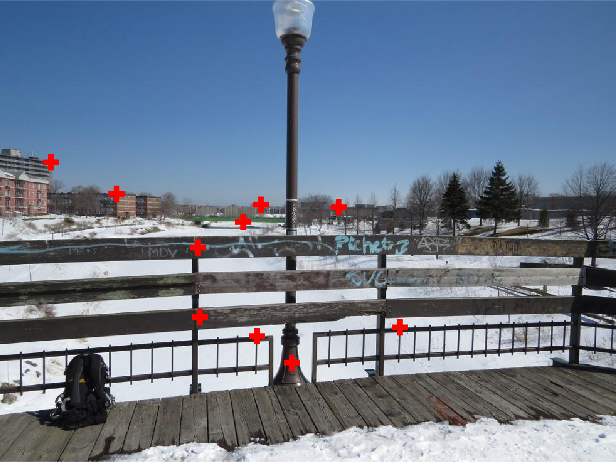
Image 3 with points related to image 2.
Here the result is similar to the previous one and also to the result presented in the assignment description. No additional points were needed aside from the ones already provided with the assignment.
Target image.
Image 1 with points related to image 2.
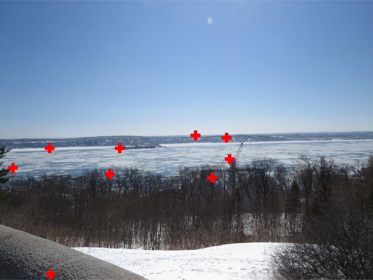
Image 2 with points related to image 1.
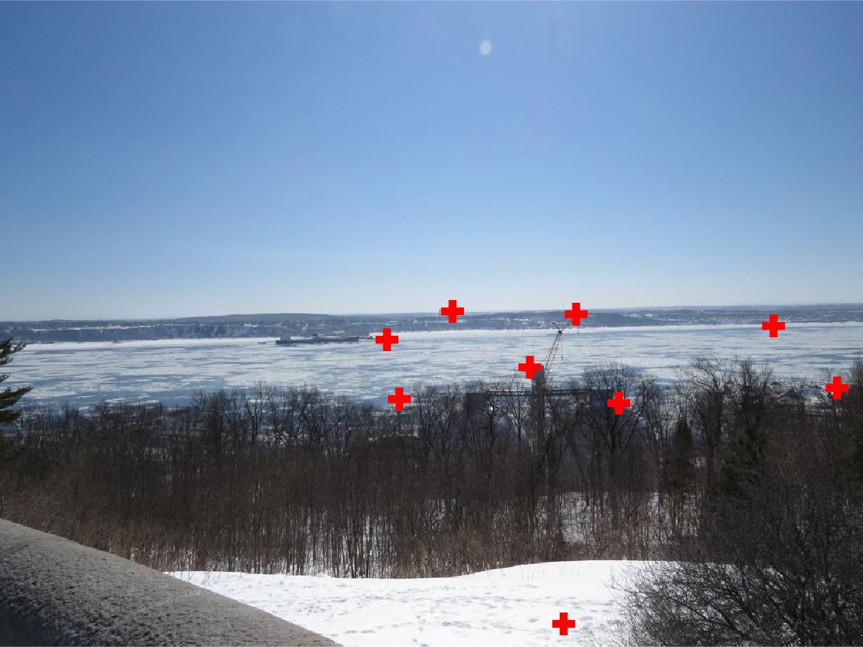
Image 2 with points related to image 3.
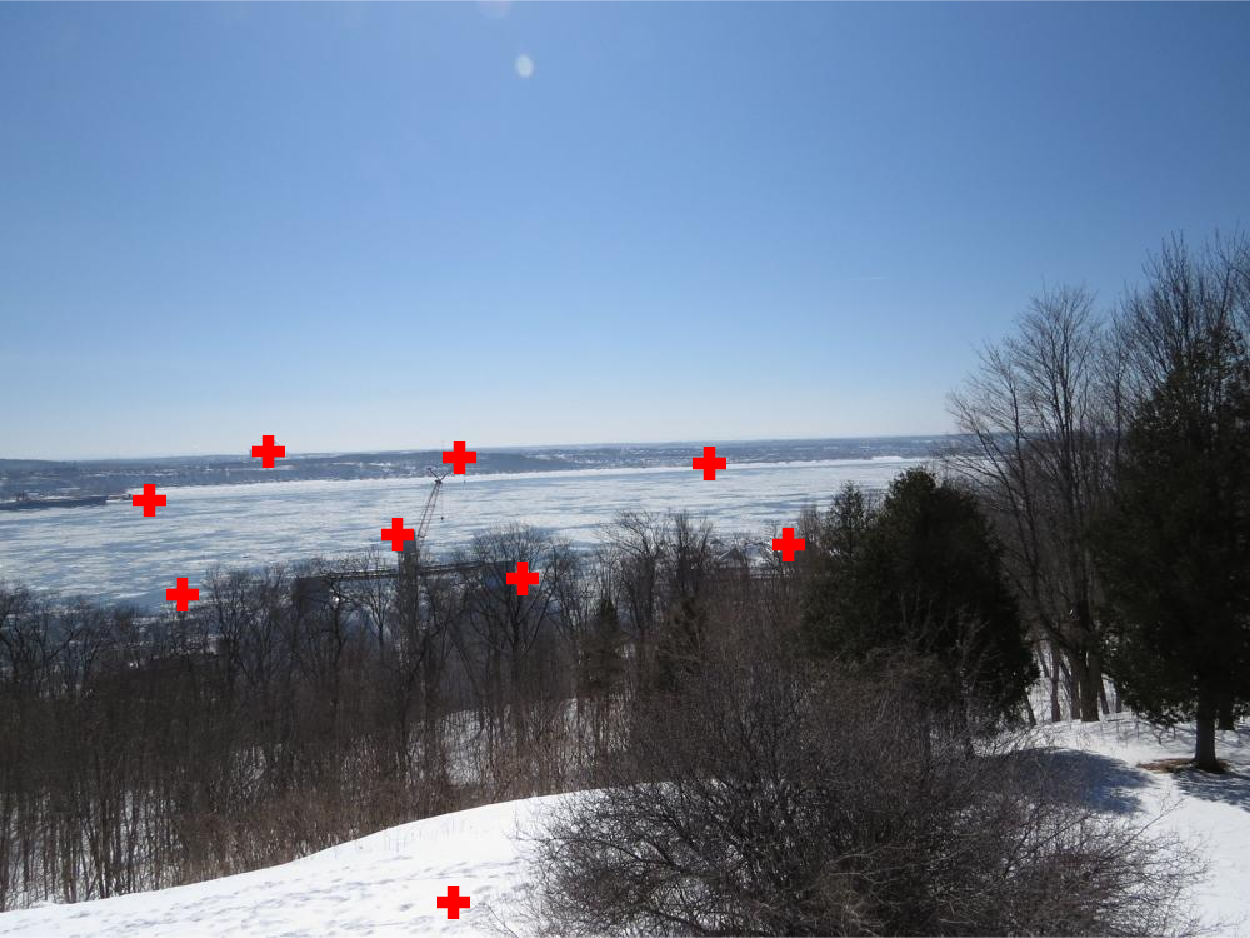
Image 3 with points related to image 2.
This serie of pictures was the most difficult one since there was no much points to match. Also many attempts did not generate a good composition, so I had to try many times until the result bellow was possible.
Target image.
Now that we are able to stitch images manually, we can go to the next step which is to do it automatically. For this we need to detect and match points on two neighbors images automatically. This apparently simple step involves many smaller procedures. First we need to detect corner features in the image using the algorithm proposed by Harris and provided as a ready-to-use code in the assignment. It creates however a huge number of points, and this is bad for performance and also for matching features points from two different images. To solve this we can use the Adaptive Non-Maximal Suppression. This algorithm works by first defining the radius from each feature point to its closest neighbor given a certain threshold on the neighbor. Points which are bigger than its closer neighbor have its radius set to infinity. After that we can pick a given number of points starting from the one with the biggest radius (which means the one that is more isolated in the image) to the one with smaller radius. In all the images I used 500 feature points. Aside from filtering the points we need to create more information about each one since they must be as much as possible distinct from each other. For that we simply take a window of 40x40 around the pixel and resize it to 8x8 in order to be less susceptible to noise. We also subtract the mean from each point inside this block and divide by its standard deviation, so that the final mean is 0 and standard deviation is 1.
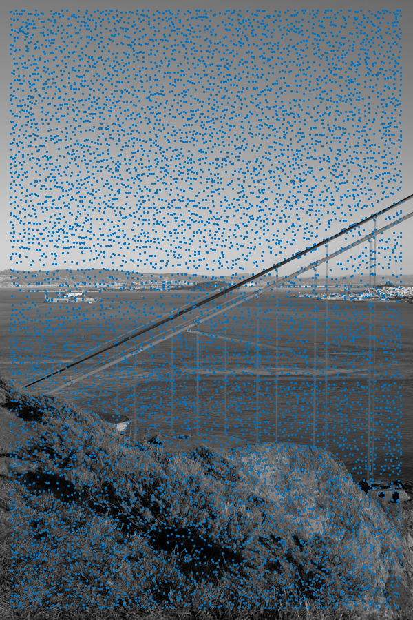
Original points obtained with Harris feature corners detector.
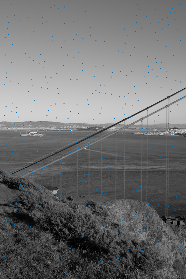
The top 500 points using Adaptive Non-Maximal Suppression.
Once we have the feature points for all images it's time to match pairs of features between neighbor pictures. For that we compare the distance from all points on one image to all points on the other image. Following the paper we use the ratio between the smallest distance and the second smallest distance between one points and its two closer "siblings" on the other picture. We also use the mean of the distance to the second closest point as a threshold to determine if a pair of points is close enough to be considered a good match.
In the images bellow we use the MATLAB function showMatchedFeatures(I1,I2,matchedPoints1,matchedPoints2); to see matchedPoints1 and matchedPoints2 over images I1 and I2.
In the sequence, we use RANSAC to find the homography matrix that best describes (given a finite number of attempts) the transformation between one set of points and the other. For that we chose 4 pair of points at random and calculate the homography matrix that describes them. Then we count the number of other pairs in the set that are in accordance with this homography given the previously mentioned threshold generated with the mean to the second closest neighbor. After a fixes number of trials (I used 100) we pick the homography that gathered the biggest number of inliers and considered it as the description of the transformation we need to perform to align the images. In the end we reuse the original pairs of inliers to recalculate the homography in order to let it more accurate.
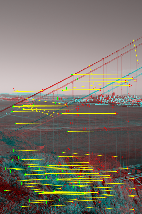
All pair of points that were considered a correct match.
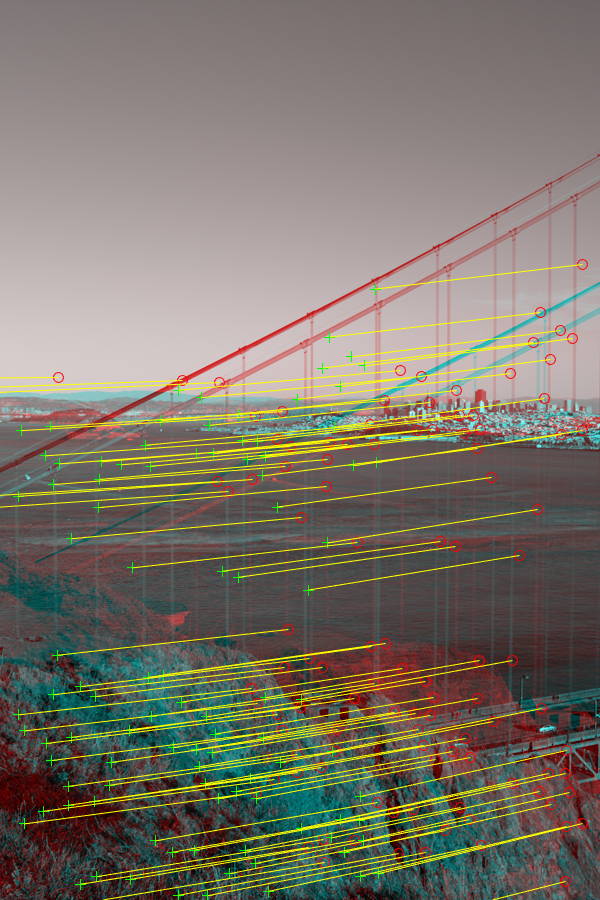
Inliers and their estimated positions given by a pass of RANSAC.
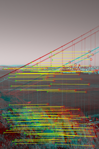
Real location of the final inliers.
The resulting panorama took time to be computed on my computer (around 5min) but the result is mostly good. Since I also used the max between two pixels to get the final value we lost part of the cable in the left of the image. The boat is also blurry but it looks like it was moving while the photos were being taken.
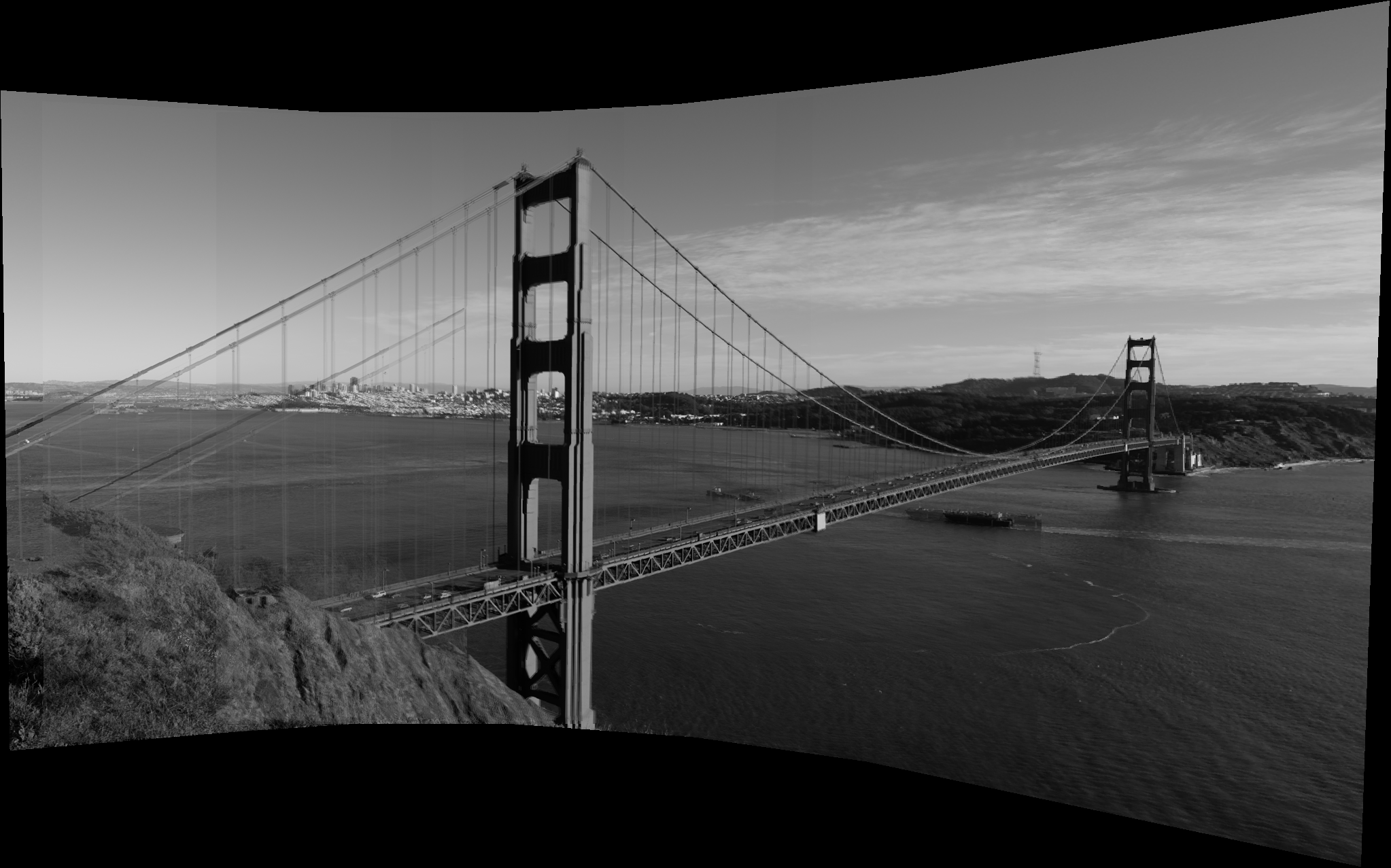
Golden Gate panorama.
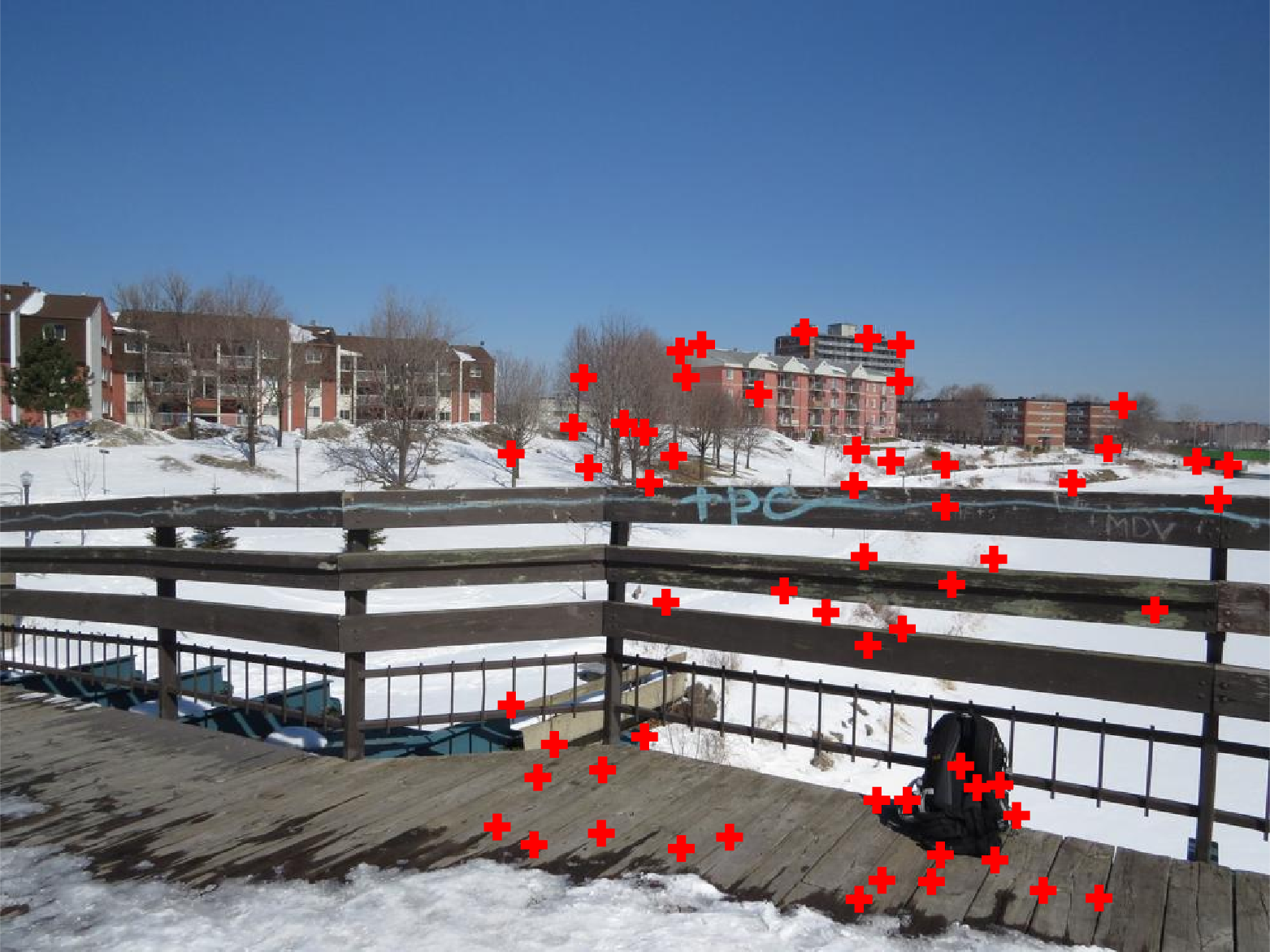
Image 1 with points related to image 2.
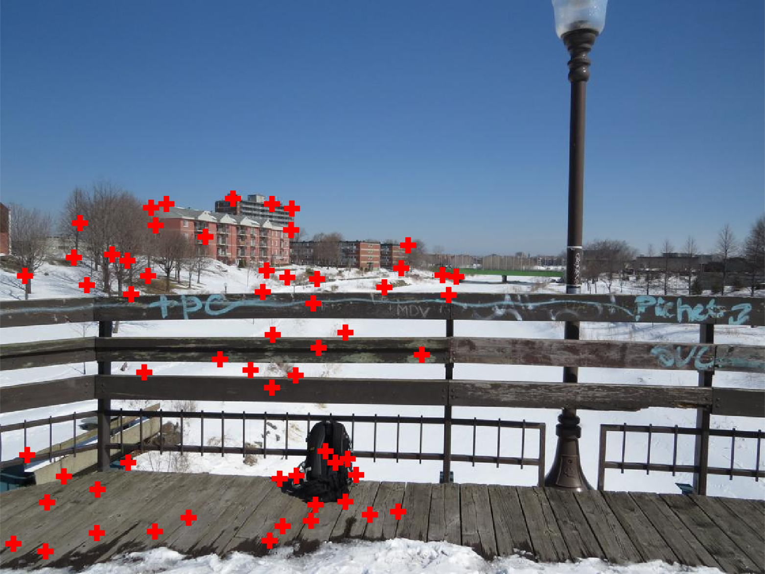
Image 2 with points related to image 1.
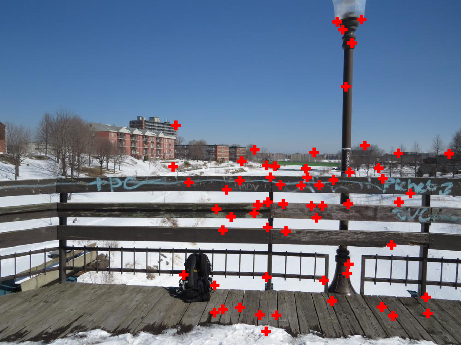
Image 2 with points related to image 3.
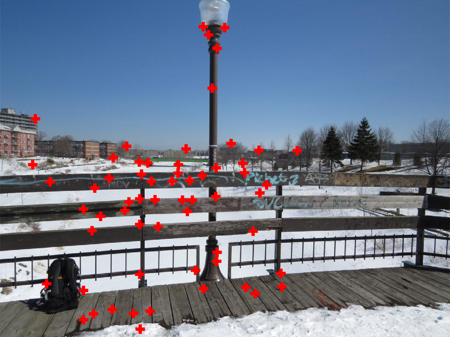
Image 3 with points related to image 2.
Above are the points that were found by RANSAC to describe the transformation. The result looks better than the one that was created manually.
Target image.
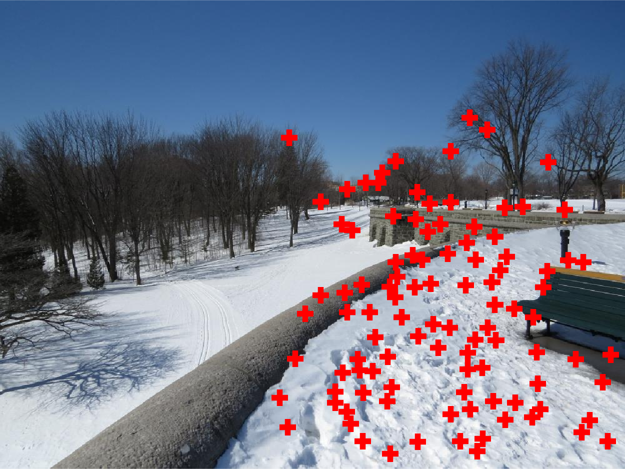
Image 1 with points related to image 2.
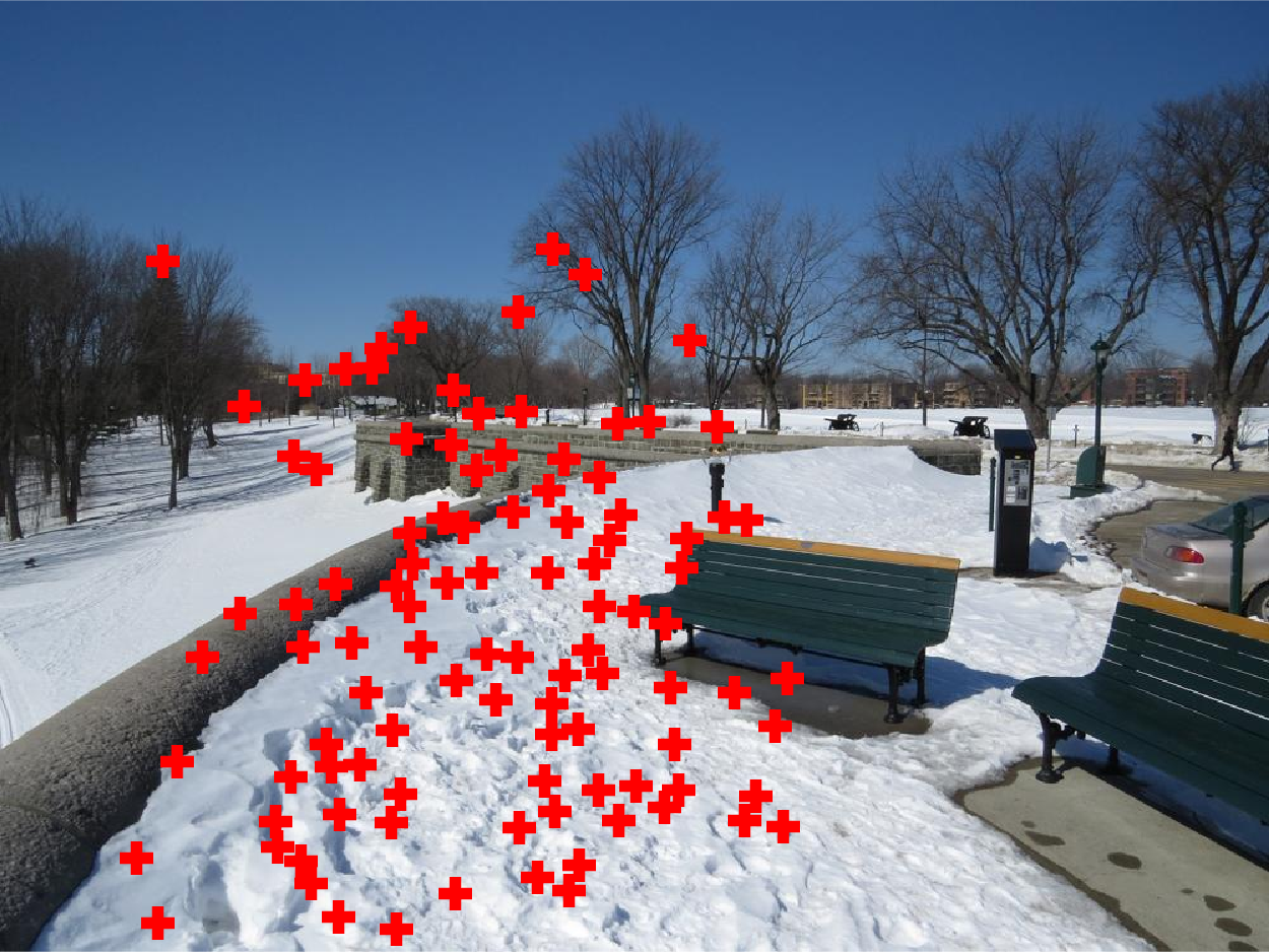
Image 2 with points related to image 1.
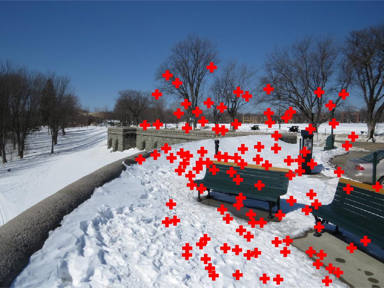
Image 2 with points related to image 3.
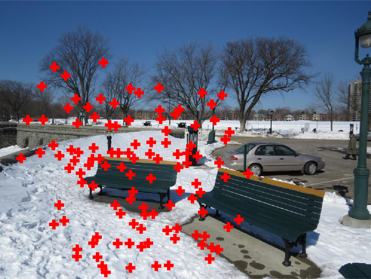
Image 3 with points related to image 2.
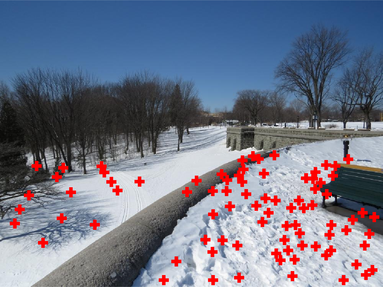
Image 1 with points related to image 4.
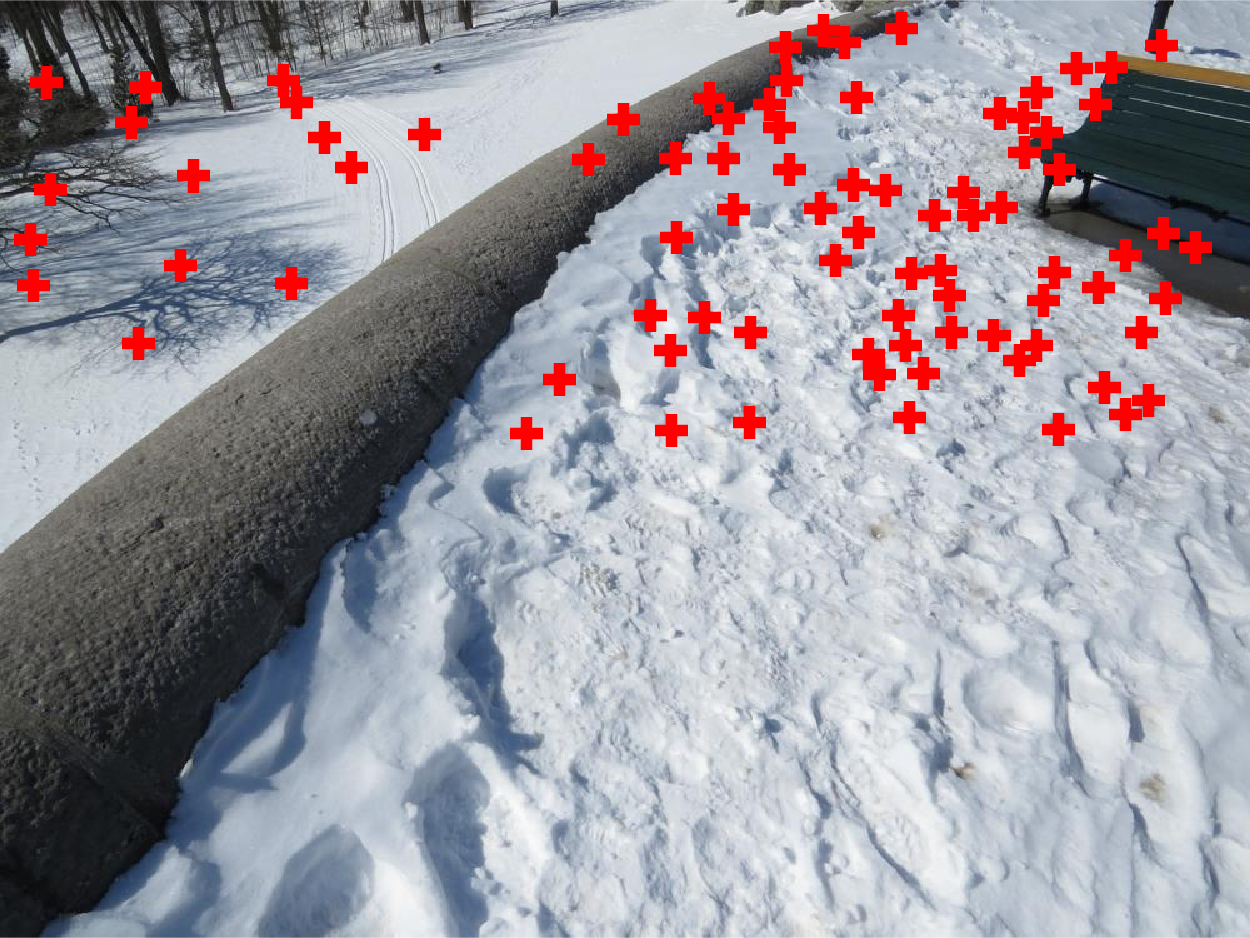
Image 4 with points related to image 1.
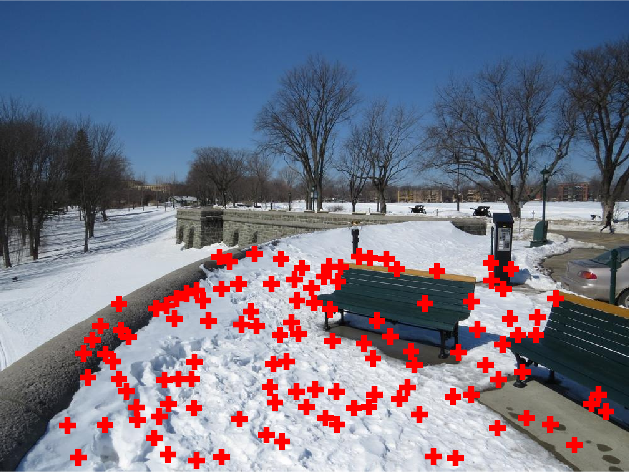
Image 2 with points related to image 5.
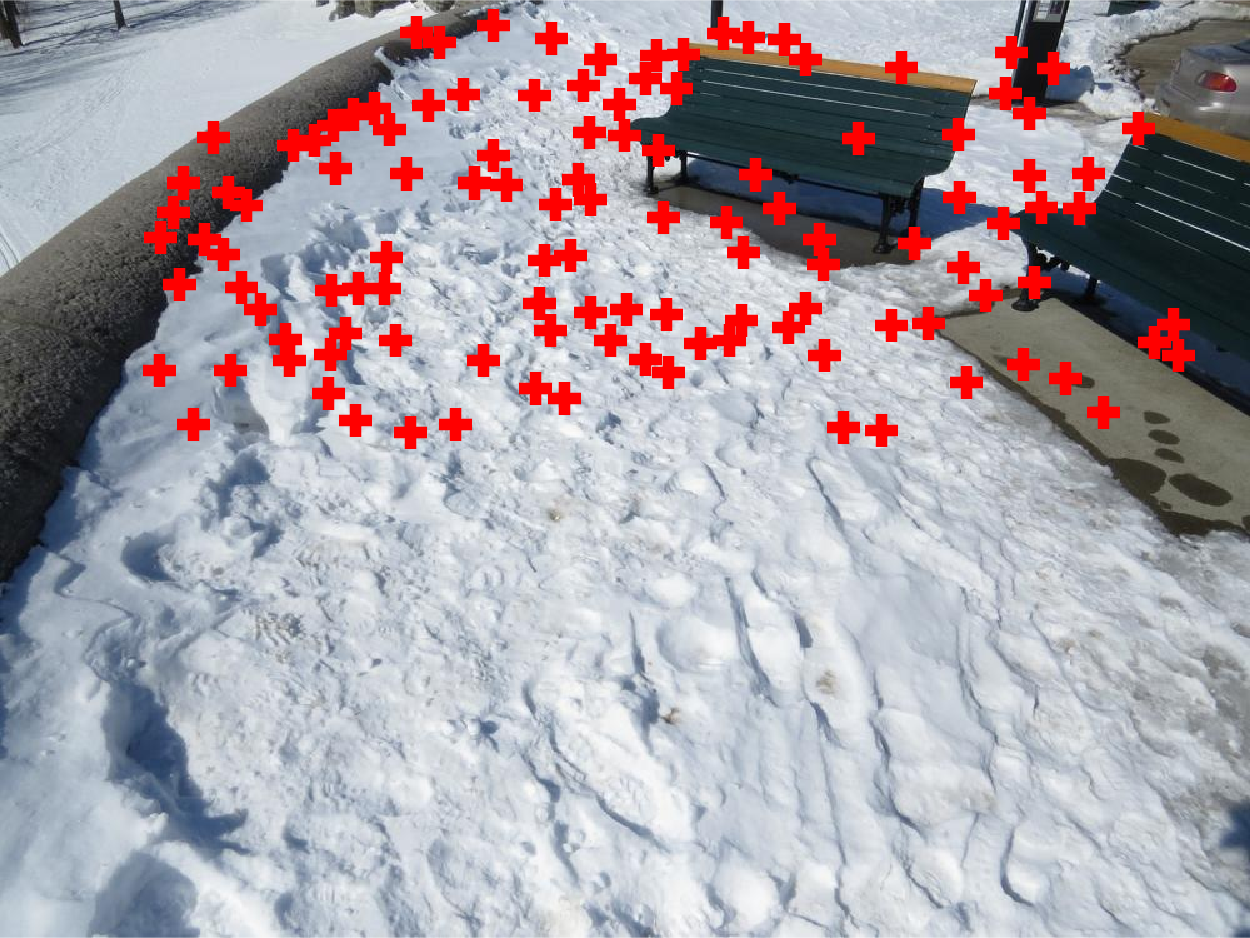
Image 5 with points related to image 2.
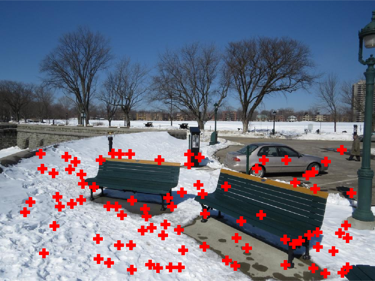
Image 3 with points related to image 6.
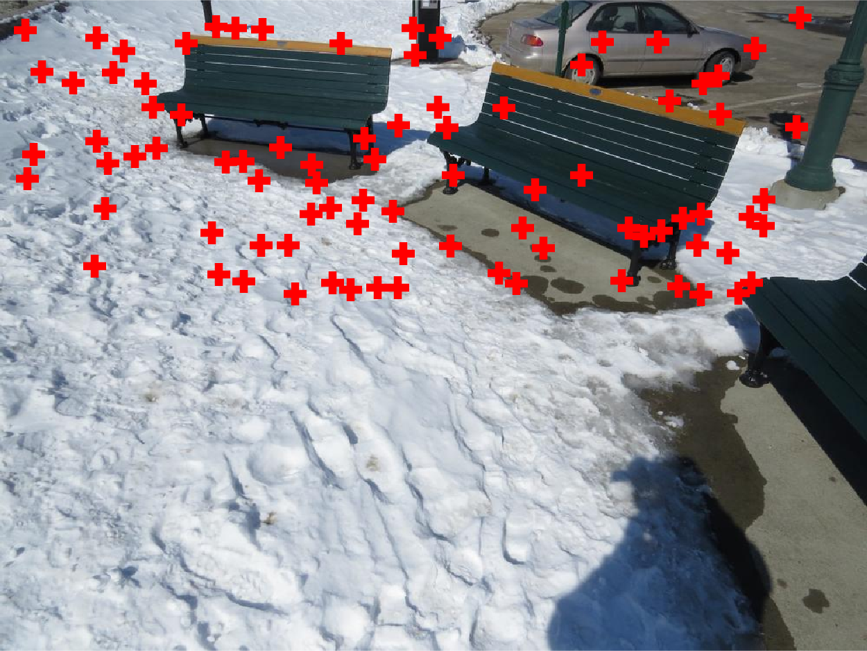
Image 6 with points related to image 3.
Here is another result with the pictures provided with the assignment. Here I average both images where they overlap, so it's possible to see the blur where they are not perfectly aligned.
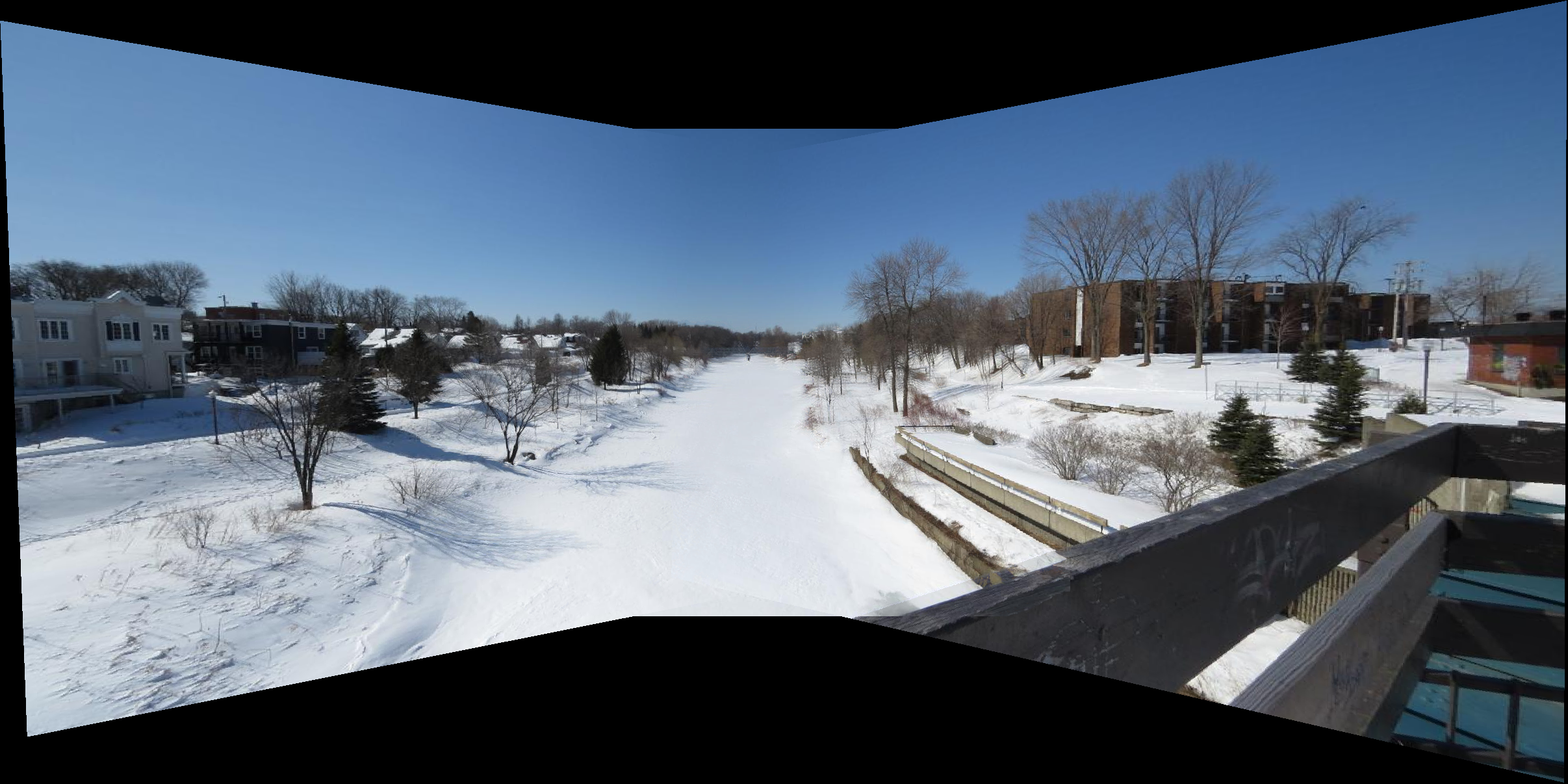
Complete panorama.
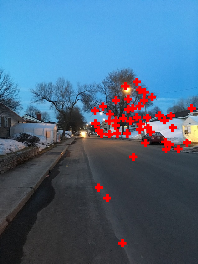
Image 1 with points related to image 2.
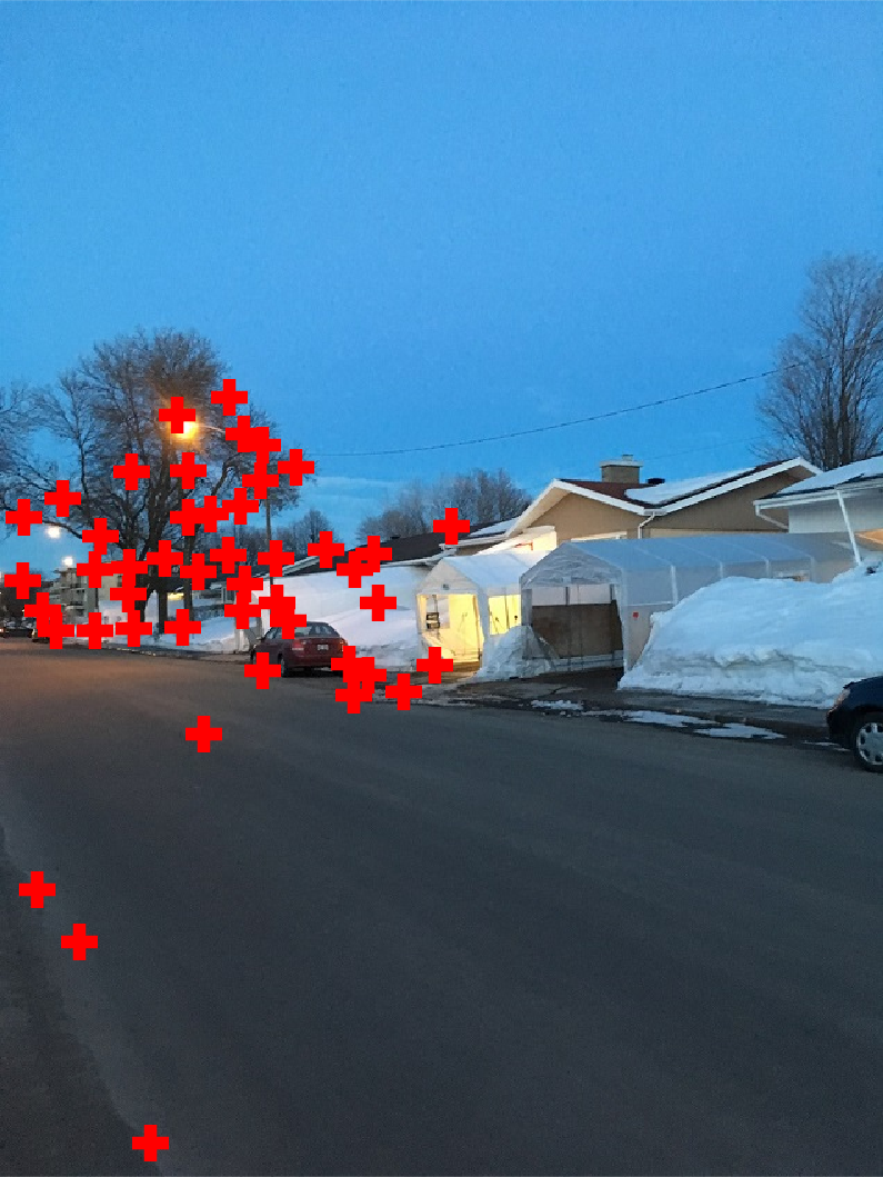
Image 2 with points related to image 1.
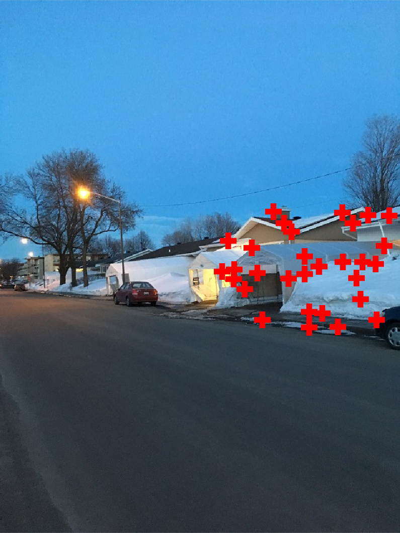
Image 2 with points related to image 3.
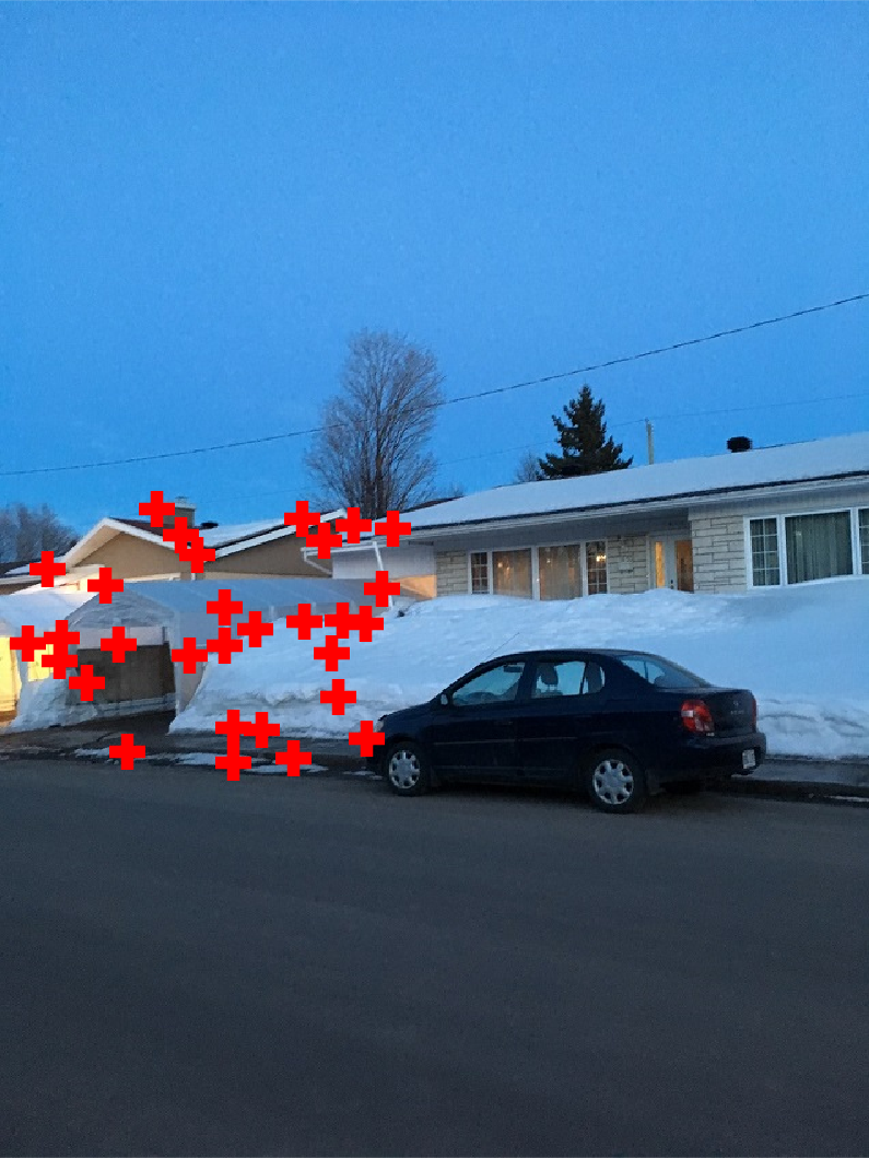
Image 3 with points related to image 2.
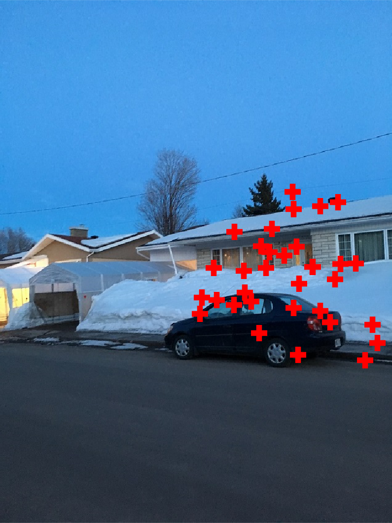
Image 1 with points related to image 4.
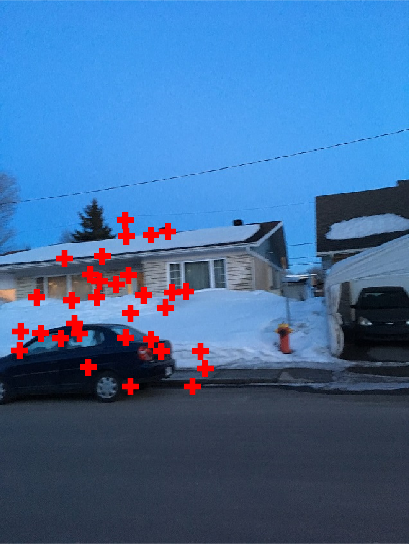
Image 4 with points related to image 1.
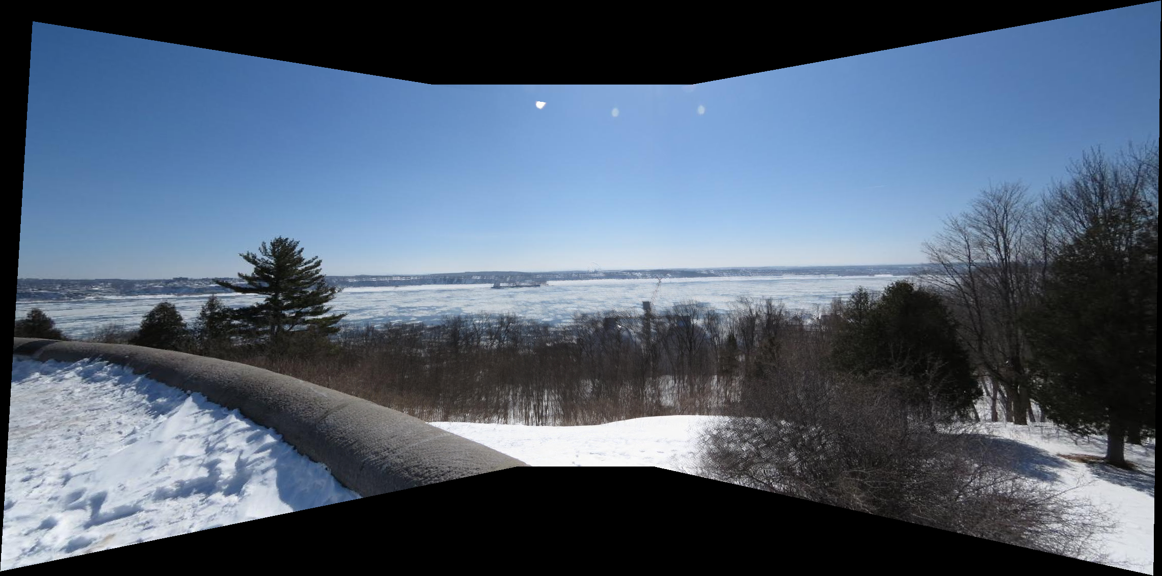
Here is one result with my own pictures. The alignment looks good and also the exposure of all pictures are similar, which helped to create a nice panorama.
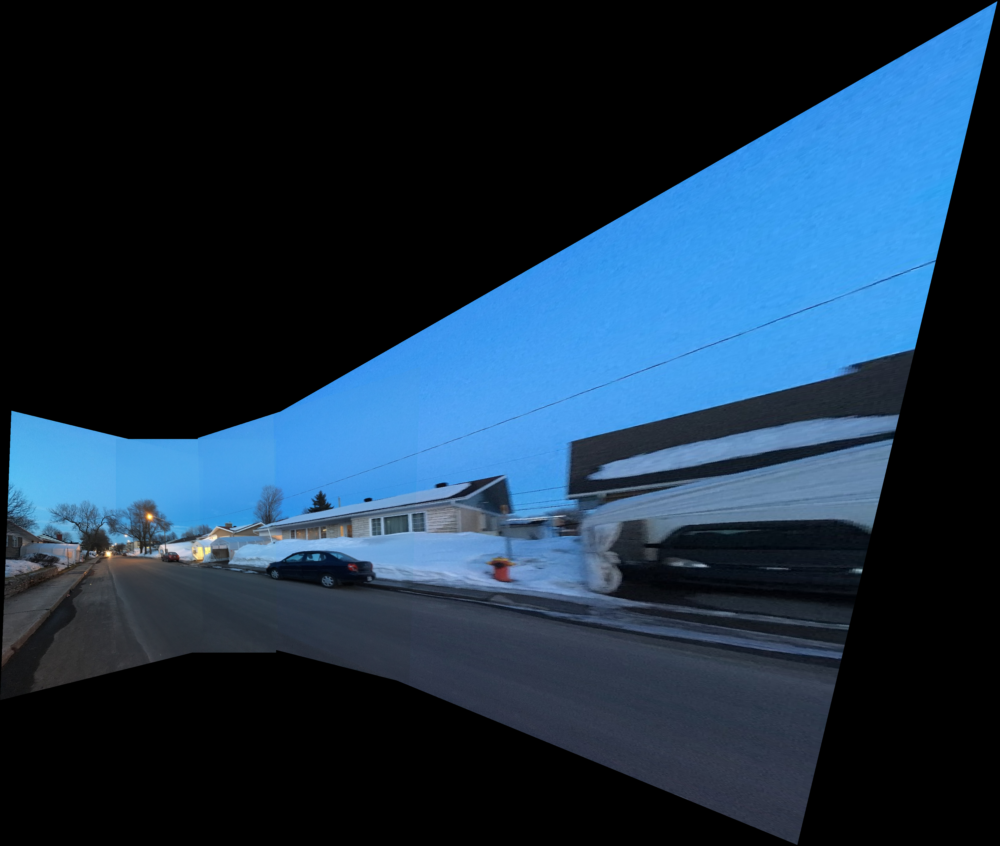
Complete panorama.
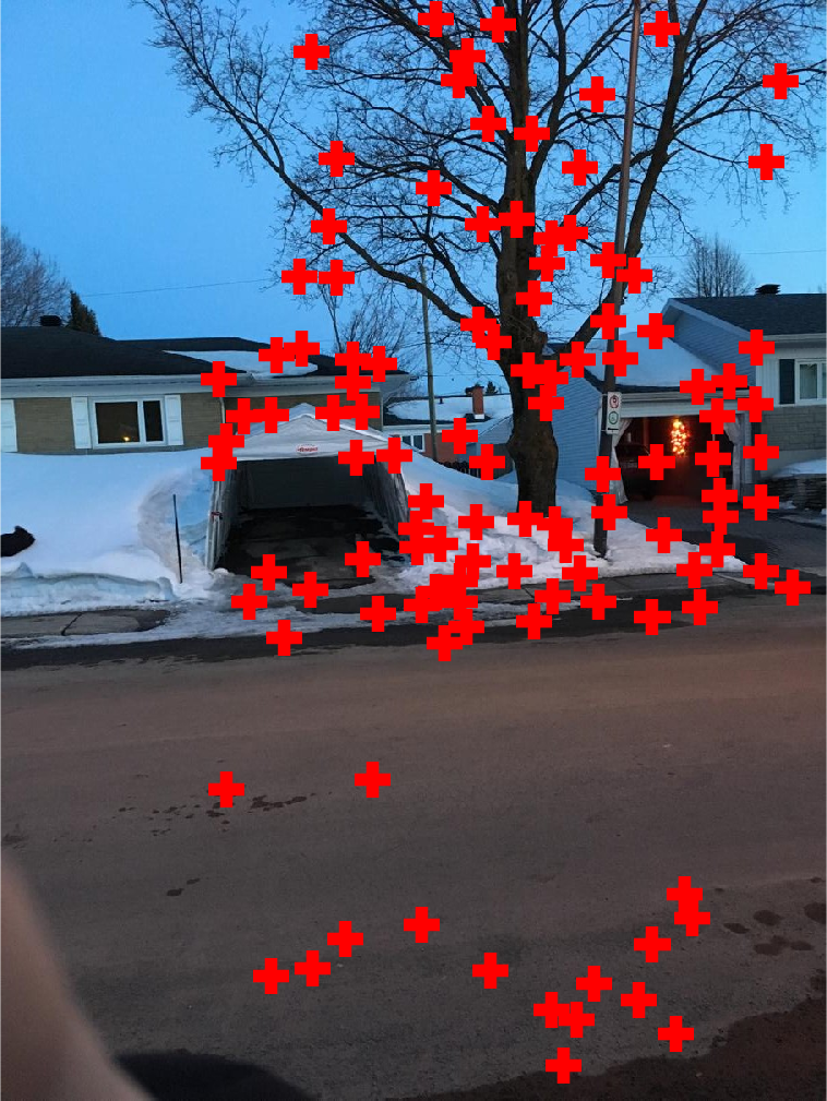
Image 1 with points related to image 2.
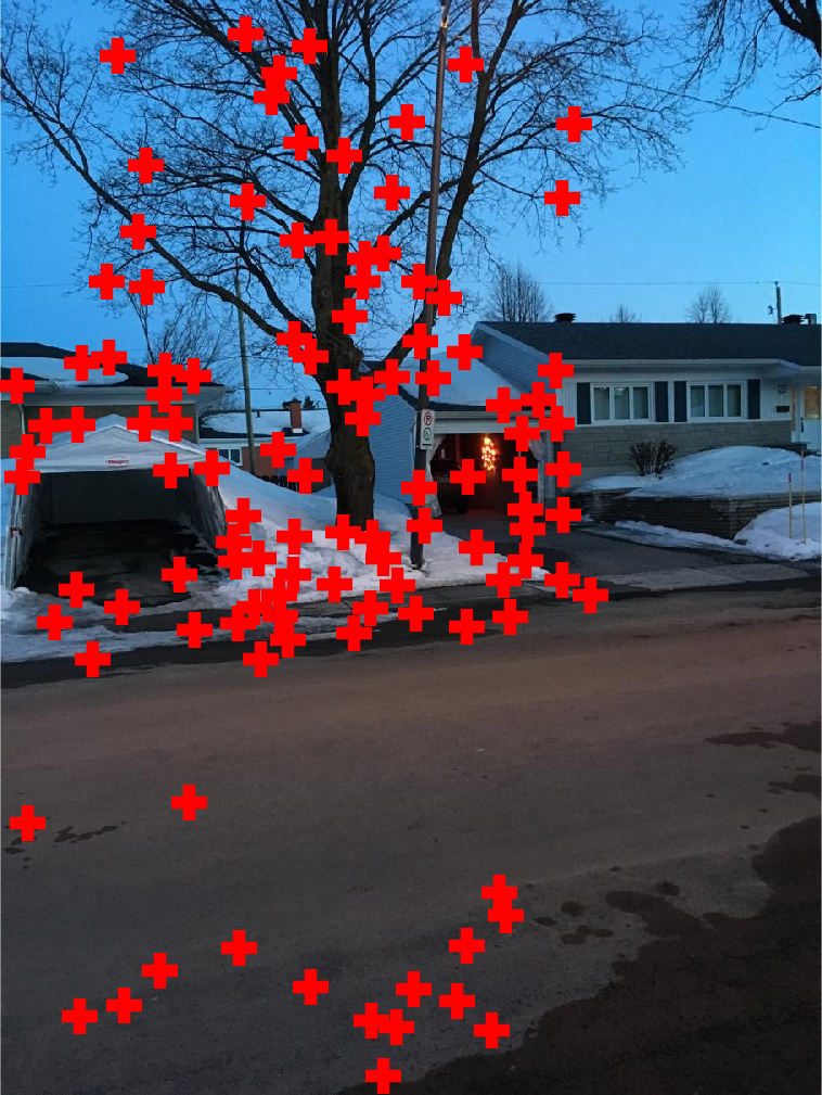
Image 2 with points related to image 1.
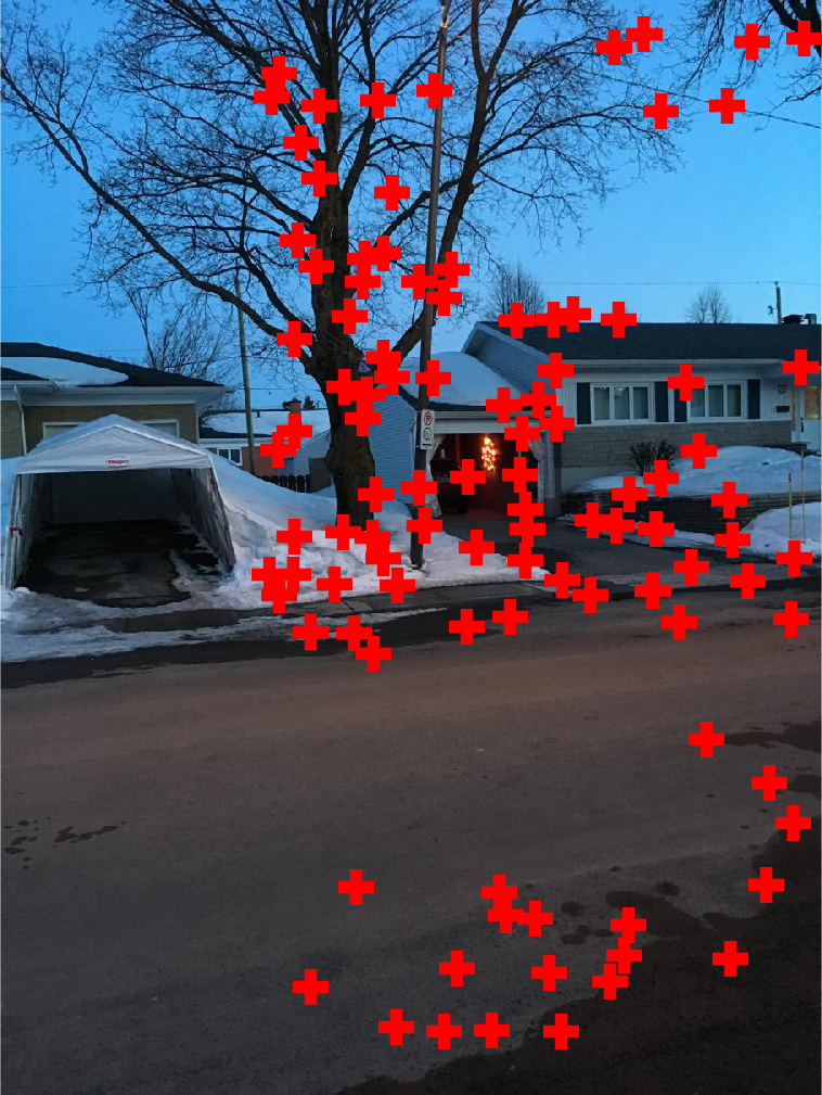
Image 2 with points related to image 3.
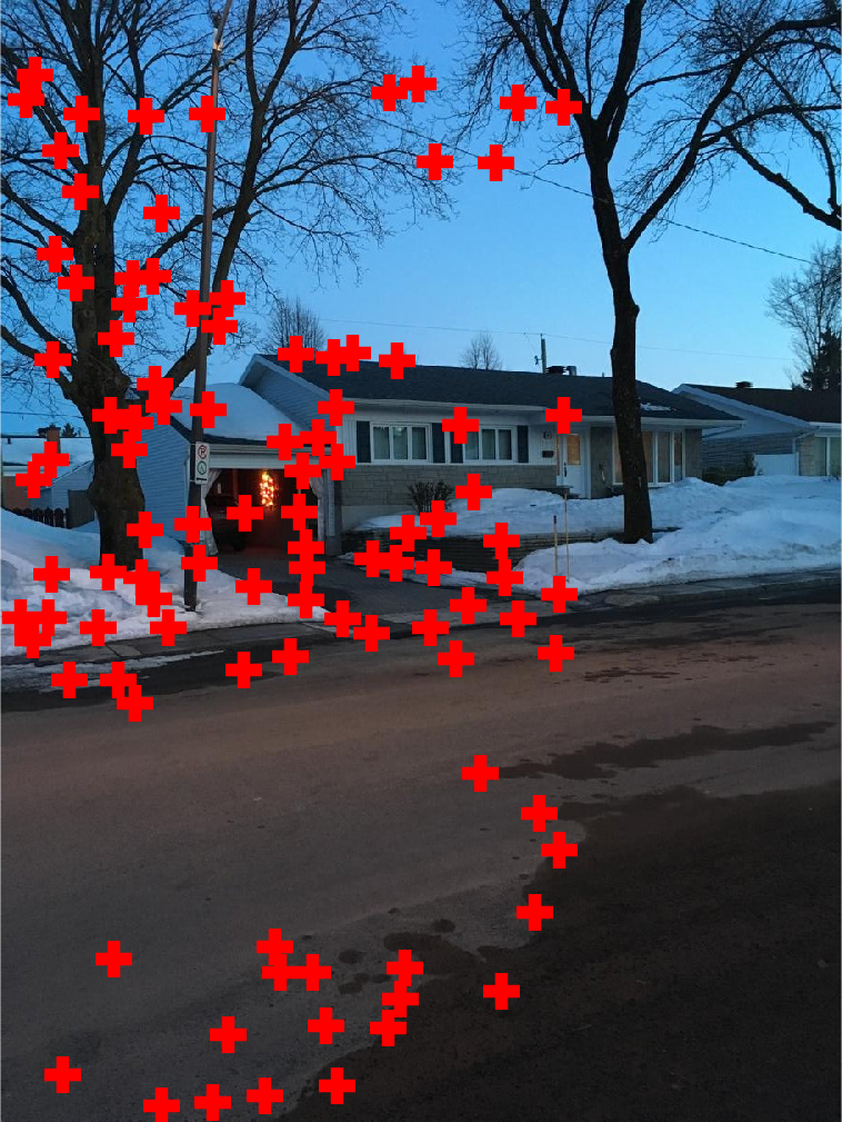
Image 3 with points related to image 2.
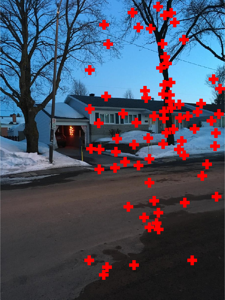
Image 1 with points related to image 4.
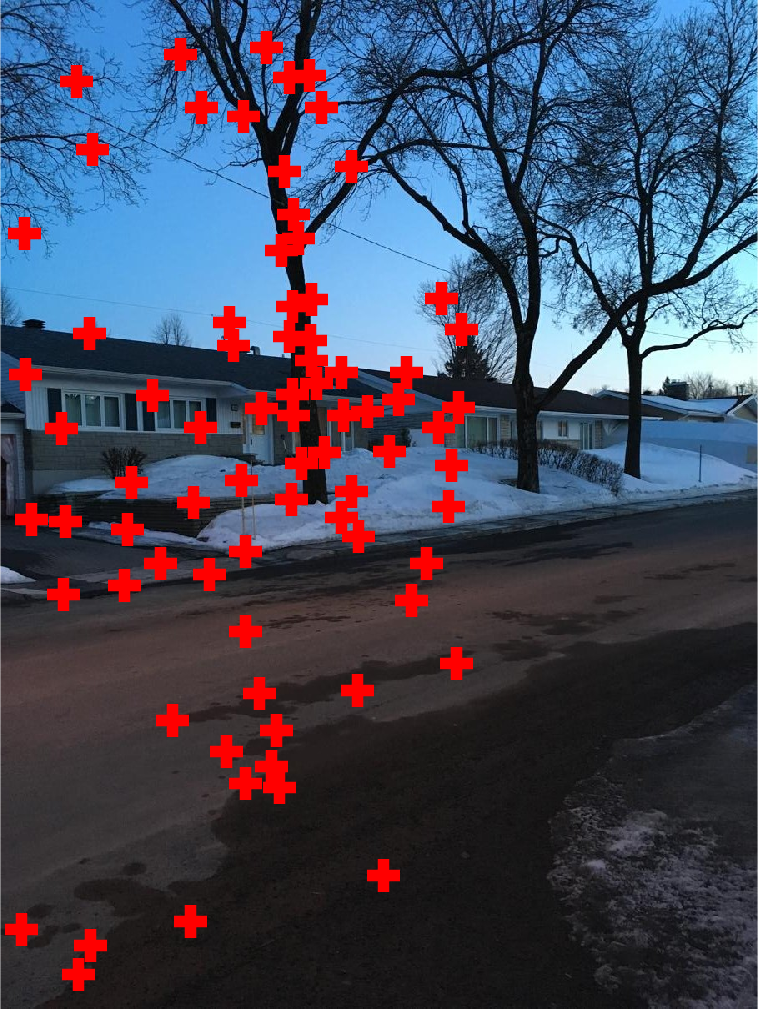
Image 4 with points related to image 1.
In this serie of photos I slowly turn around the camera, which gives a better result (which can be seen by the borders that are well alligned).
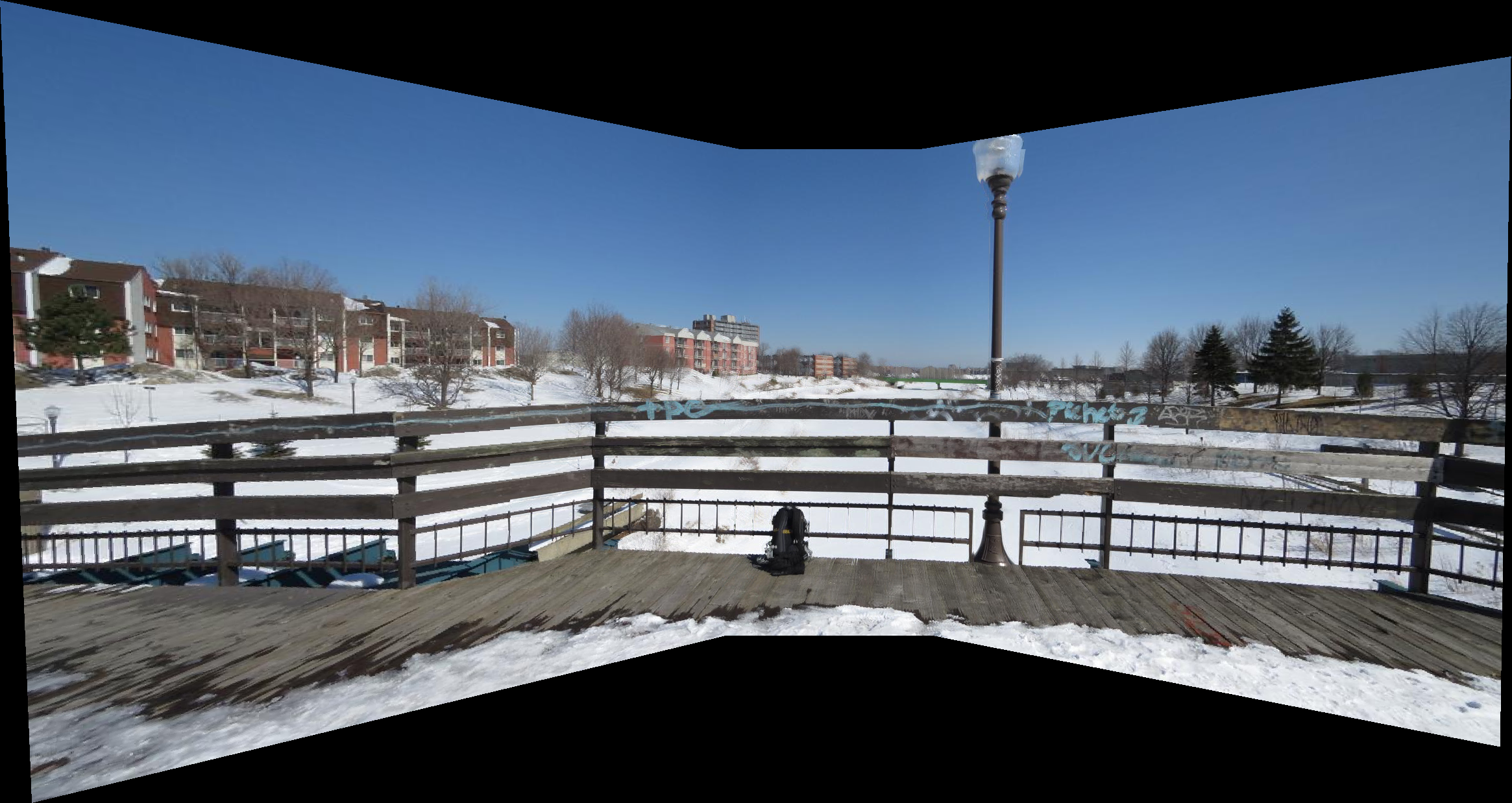
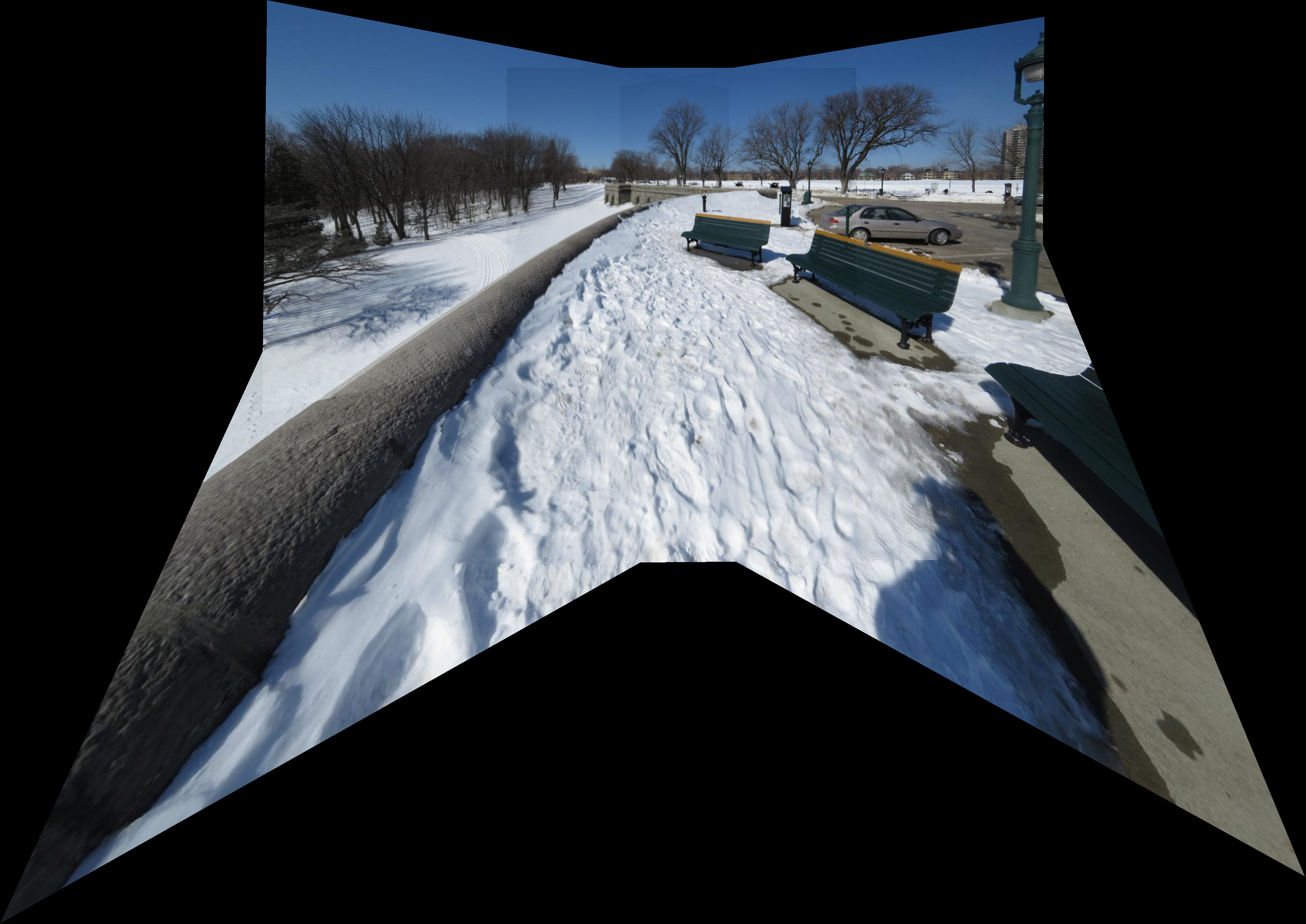
Complete panorama.
To place the picture in the right place it was enough to define the four corners in each image and then compose them.
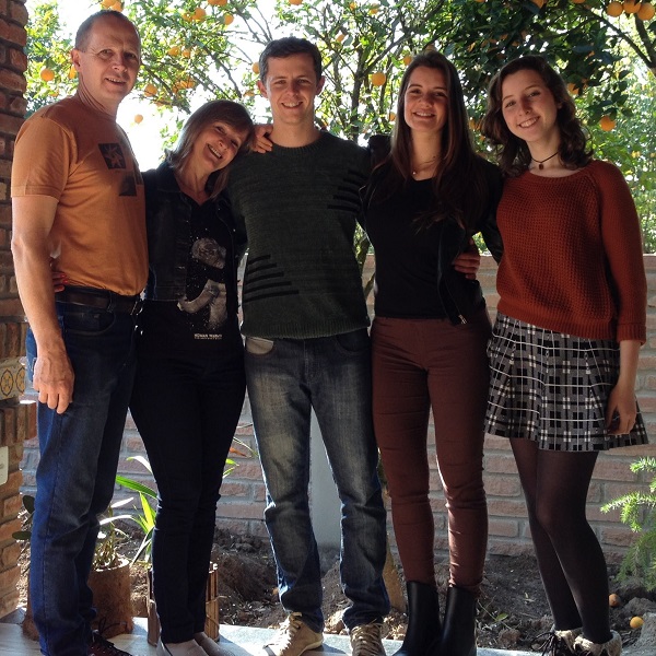
Photo of my family.
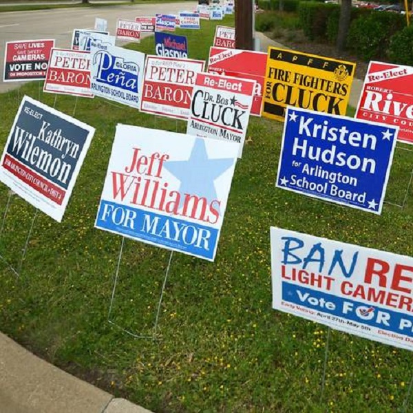
Signs.
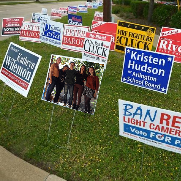
Final composition.
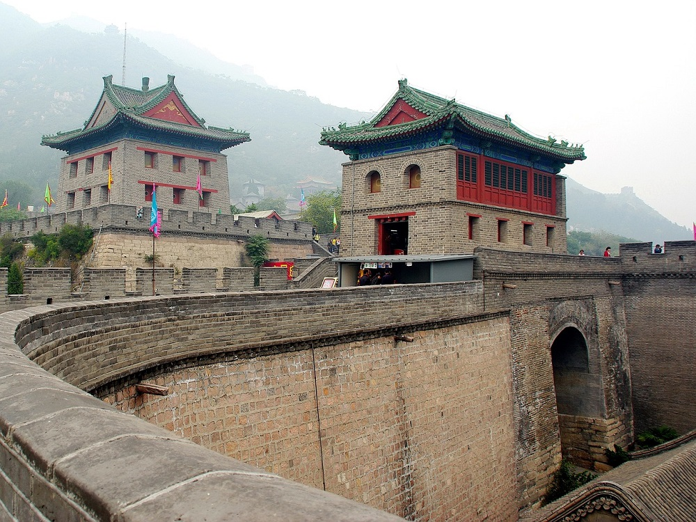
Here the grafitti was composed in a wall. To use only the grafitti the background was set to black, so when we compose them we can ignore the background.

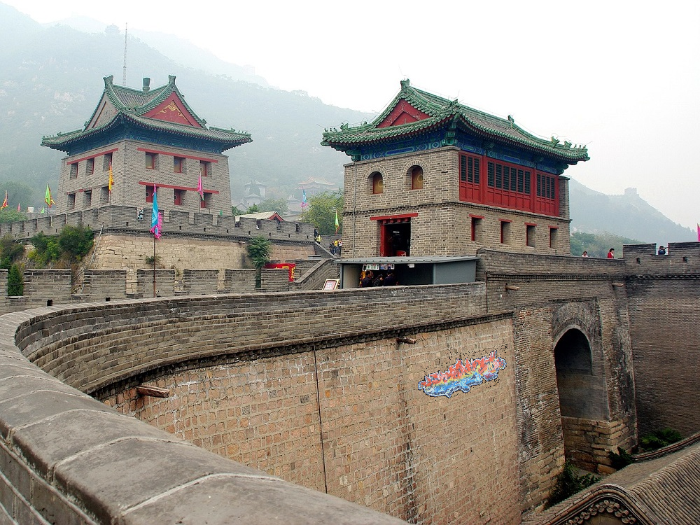
Some place in China.
A grafitti.
Final composition.