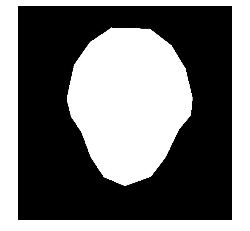
Where the visage mask of the first image Im1 is:
Algorithm
The implementation follows the guideline declared in the lecture. The algorithm needs following datasets/variables:
1. Im1: first image which is the starting point of the morphage
2. Im2: second image to which the first image is morphed
3. img1_pts: correspondence points in image 1
4. img2_pts: correspondence points in image 2
The pipeline then was implemented as follows:
1. calculate triangulation
For each intermediate morphage stage:
2. calculate intermediate triangulation
3. for each triangle, calculate the transform in direction of Im1 and Im2
4. for each pixel within the triangles in Im1 and Im2, interpolate the color from the original image
5. add background
The triangulation was calculated using Delaunay-Triangulation. Furthermore, the triangulation was calculated on an intermediate morphing stage as it should be a good
triangulation for both original images. The intermediate triangulation was calculated using the corresondence points
and bases on a linear interpolation between the to images of the form:
img3_pts = warp_frac * img1_pts + (1-warp_frac) * img2_pts (I)
In this case, warp_frac was set to 0.5. The same formula later was used in step 2 for the calculation of the intermediate morphing stages.
Triangulations assigns the number of the triangle to which a pixel belongs to every pixel in the image.
The idea then is to perform local transformations, i.e. transform the triangles rather than to apply a global transformation on the entire image.
In this exercise, an affine transformation should be applied (step 3). This transform has 6 degrees of freedom, thus, 6 equations need to be established to resolve
the system. 3 correspondences, corresponding to the 3 points of each triangle, are needed to establish the system of linear equations in order to define the transformation:
a = T * b (II)
where a are the resulting coordinates from the transform (thus img3_pts of the intermediate triangle), b are the points of the original image (img1_pts and img2_pts, respectively), and T is the affine transformation.
In Matlab, this system can be resolved by:
T = a\b (III)
For each pixel, the color value then has to be found in the original image. This is done based on a backward-transformation, i.e. for each pixel in the
morphed image, the position in the original image is calculated, where the respective pixel in the new images derives from. As this backward-transformation might
result in inter-pixel values (i.e. we might get a position between two pixels), the intensity-values of the morphed image are calculated based on a bilinear
interpolation. In order to reduce calculation time, step 4 was applied seperately on every subset of pixels belonging to a triangle. The respective pixels
could be found using mytsearch. The final pixal value is a combination between the interpolated pixel values from Im1 and Im2, where the wheigt of the two
input images depends on the stage of morphing.
Finally, the background was added. I first set here 4 additional corresponding point into the corners of the image. For this points, I again calculated a triangulation and
following the same approach as for the morphed objects. However, the pixel in the morphed images only was filled with the calculated backgroun intensity, if the
pixel did not belong to a triangle.
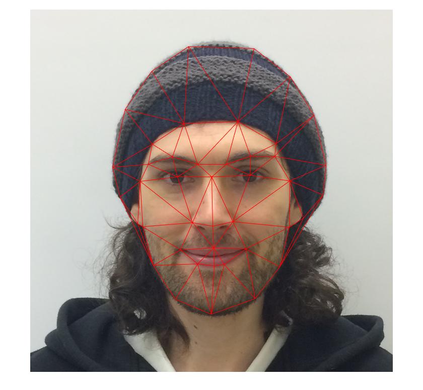
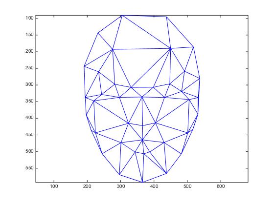
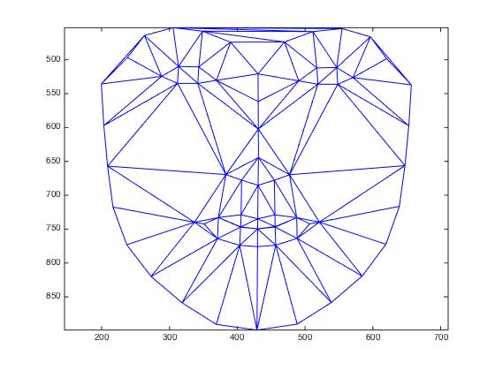
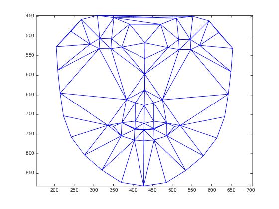
First, the triangulation was set up. This looks as follows:
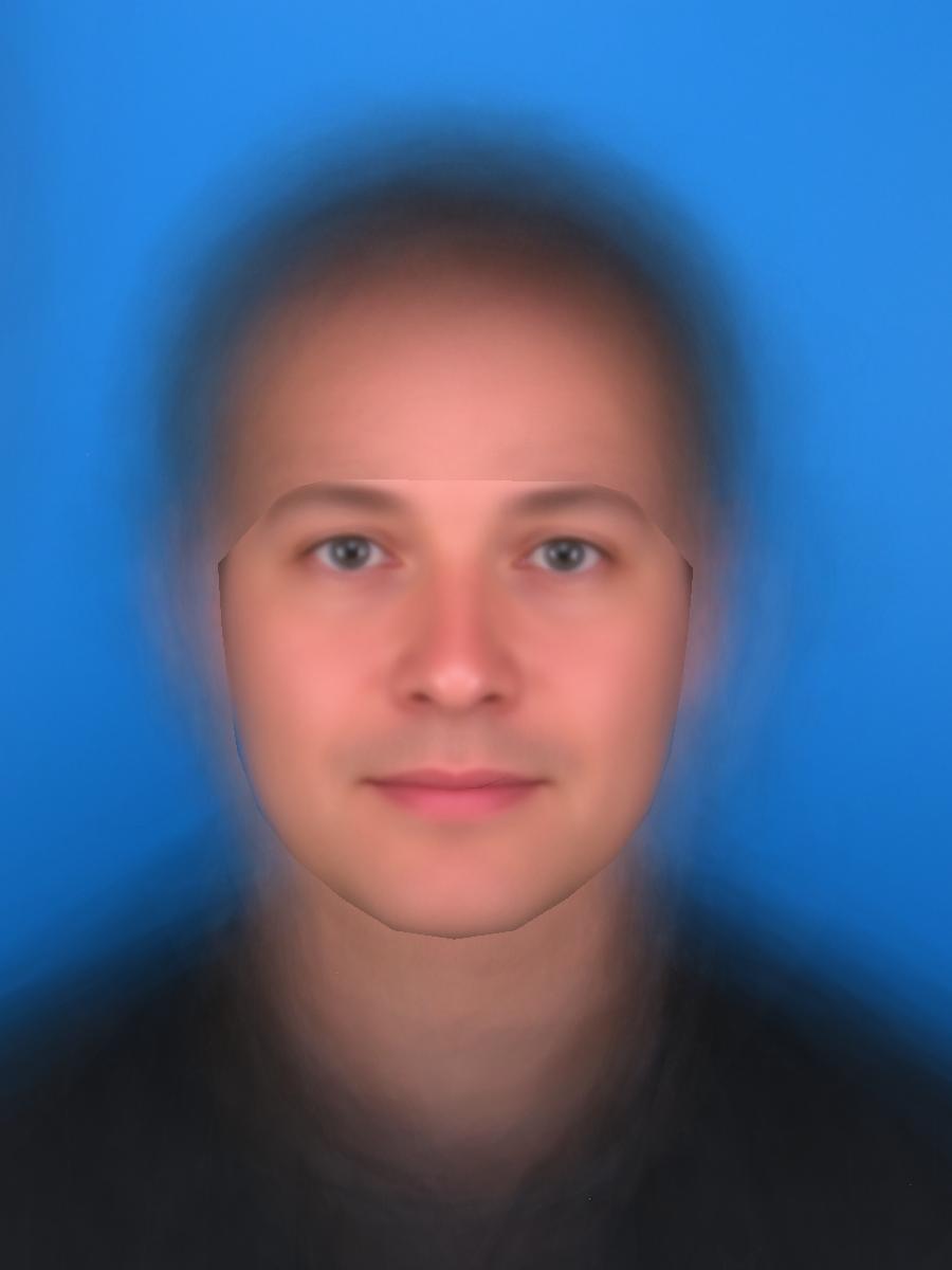
Where the visage mask of the first image Im1 is:
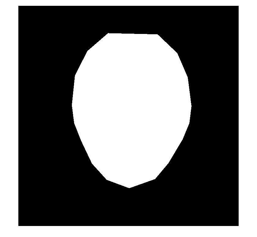
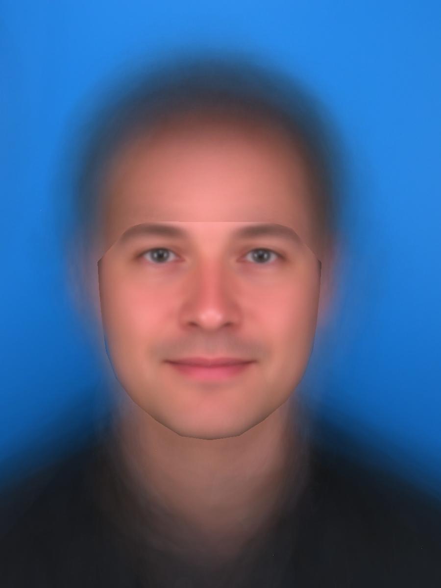
and the morphed visage mask at an intermediate stage is:
The resulting visage morphing looks as follows:
| 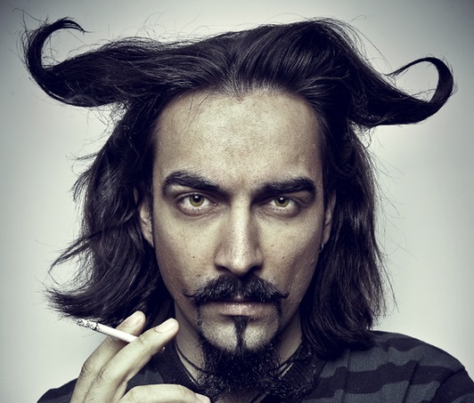
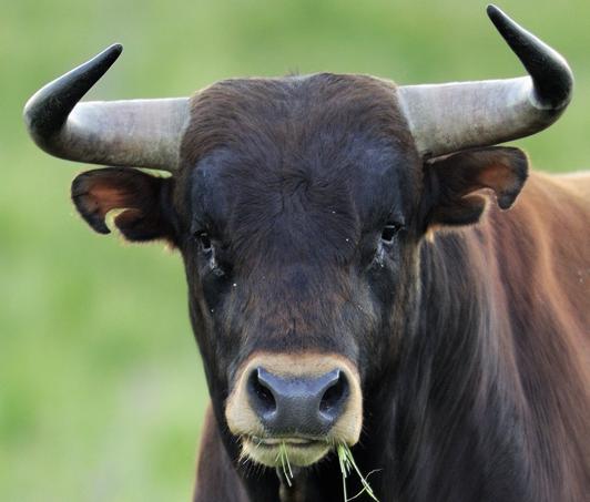
| source bull: http://weknowyourdreams.com/images/bull/bull-07.jpg | source devil: http://www.portrait-photos.org/_photo/3181255.jpg |
|
Another example is the transformation between animals, in this example the morphing of a lion into a tiger:

| 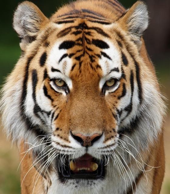
| source lion: http://res.cloudinary.com/hrscywv4p/image/upload/c_limit,fl_progressive,h_1200,q_90,w_2000/v1/178274/The-best-top-desktop-lion-wallpapers-hd-lion-wallpaper-11_xjbx08.jpg | source tiger: https://mynicetime23.files.wordpress.com/2014/09/tiger-face-16.jpg |
|

| 
| source trump: http://www.calbuzz.com/wp-content/uploads/Donald-Trump.jpg | source frog: https://fanart.tv/artist/3df914b9-e0bc-493c-875a-c412f84ecdad/crazy-frog/ |
|
| 
|

|
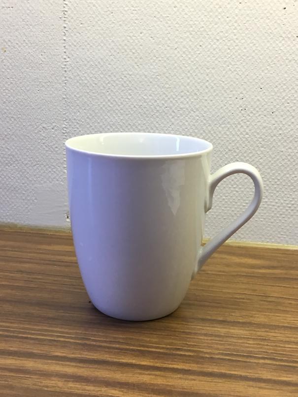
Another example is morphing of a kettle into a cup:

| 
|
|
Discussion
As seen, the morphing algorithm works for visages as well as for objects. The contours are
transformed into each other as demanded.
However, two requirements have to be fulfilled
in order to achieve this results. First, an adequate number of correspondences has to be
defined in both image. Definition of the adequate number is not always easy to define and highly depends
on the object. For example, morphing of devil/bull was achieved based on 49 correspondences instead
of 43 as for the visages.
Second, care has to be taken that the arrangement of corresponding points in both images is
comparable and of equal order. Equal order is mandatory as only this proceeding ensures a correct morphing.
However, in the examples above, some deficiencies can be recognized. A first deficiency
relates to the background/background definition. Background definition is not always very
obvious, as for example for the lion and the tiger. As the mane of the tiger fills a large part of the
image, I considered some amount of it as background. However, this approach was not too wise.
The same can be seen for the devil, who's hair I considered as background, like I did the body of the bull. This
reduces the morphing effect.
Another problem affects the blending of the intermediate morphing stages. I chose the weights
according to the proportion of the stage, defined by warp_factor in equation (I). However, the second images
appears to fast while the first image disappears to slowly in morphing. A wiser decision might be
found here.
Crédits supplémentaires
Morphing of hybrid image
Methods
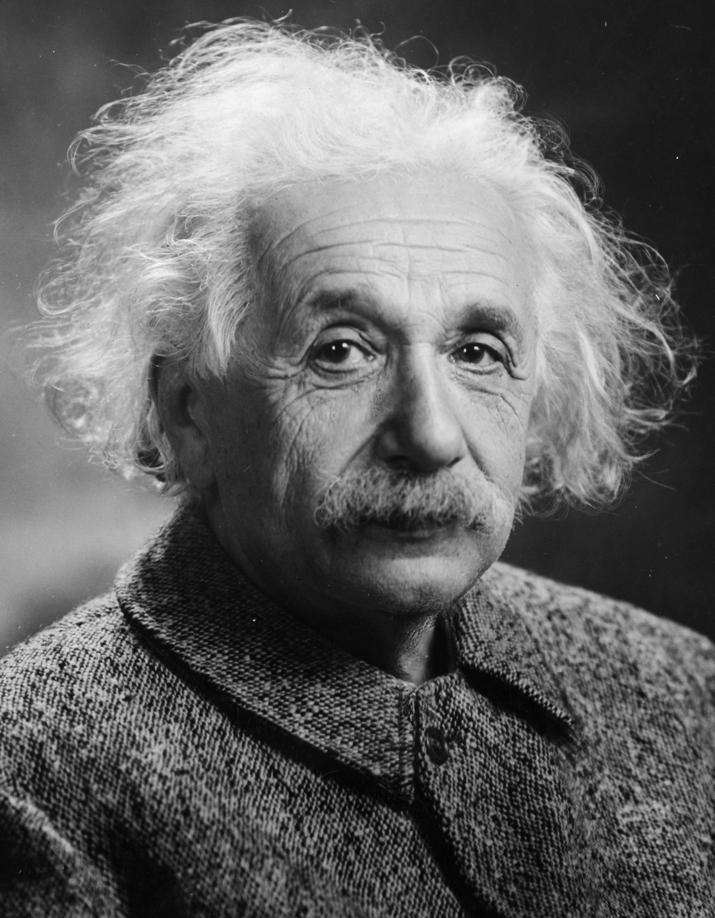
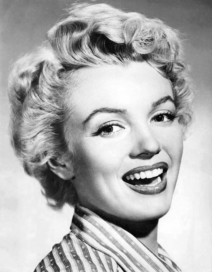
In this example, a hybrid image as intermediate stage in morphing is created. That for,
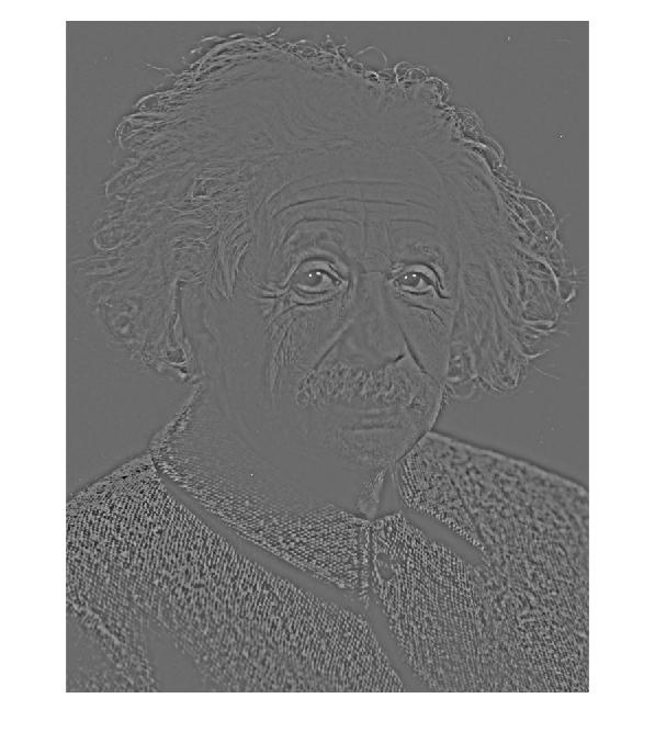
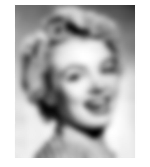
a high-pass filtered image (Einstein) is morphed into a low-pass filtered image (Monroe). While Einstein
is visible at first, his portrait is morphed into the one of Marylin Monroe, where the intermediate step corresponds
to the hybrid image.
Filtering of the images was done as described in TP2 (same thresholds for the filters) and image morphing
was done using the algorithm from above.
Results The input images as well as the results from morphing are presented in the figures.
| original Einstein | original Marilyn |
| 
|
| high-pass filtered Einstein, normalized | low-pass filtered Marilyn, normalized |
| 
|
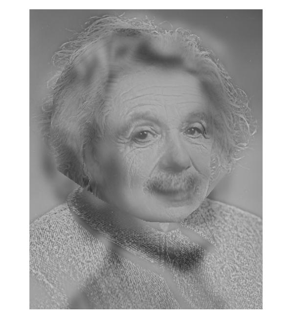
| animation | intermediate stage |
| 
|
Discussion The morphed hybrid images is not as good as the hybrid image from TP2. The region in the image, within which the hybridization works fine, is limited to the area defined by the correspondence points, while for the background, the hybrid image is affected by the parameter defining aggregation of the two images, namely the variable dissolve_frac. The morhped and hybridized image region, which is reduced to the visage, thus, visibly stands in the foreground at the intermediate stage, showing distinct edges to the background. This lowers the effect of hybridization.
Polar coordinates
Methods The approach here is the same as for cartesian coordinates. Homogenous polar coordinates are of form [theta, rho, w].
Vector-field based Morphing
Methods Instead of transforming triangles, where the idea is to perform local transformation, one could find specific transformations for every pixel. The workflow looks as follows:
1. find displacements between the corresponding points, i.e. find desired displacement between
the corresponding point in the original images and the target image (morphed image)
2. calculate distances from every pixel to every correspondence point
3. calculate a vector field by interpolation
4. specify the transformation for every pixel
Step 1 results in the displacement vector between the corresponding points in the images. For each
correspondence pair, the respective vector can be calculated as:
[dx, dy] = [(x_p1,target-x_p1,original), (y_p1,target - y_p1,original)];
As vector field interpolation should be weighted, the distance for every pixel to every correspondence point was calculated in step 2. This distances are used in step 3 for the interpolation, where the weights for every displacement vector of the correspondence points are chosen as the inverse of the squared difference to a pixel, normalized by the total sum of distance. Finally, the calculated displacement was applied for every pixel.
Results The figure shows the result from pixel-wise displacement based on interpolated vector field. Here, I used the portraits from task 1.
![]()
Discussion
The implemented algorithm works in principle, the portraits are morphed. However, interpolation
of the vector field shows some deficiencies, resulting in some hard breaks where portraits show some
breaks. Clearly visible are the correspondence points around which morphing works fine. On the other
hand, only parts within the visages are affected, while the general outline of the heads transforms well.
Overview
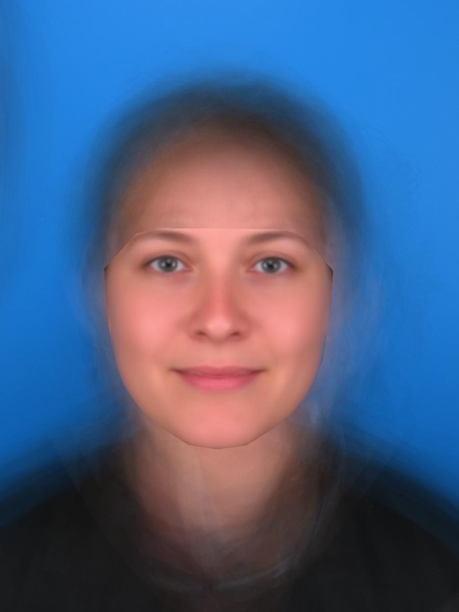
In a second part, we want to calculate an average face based on the Utrecht data set which
contains a total set of 131 portrait photographs of 68 men and 63 women. Furthermore,
the average male and female face is calculated in order to masculinize and feminize my own
portrait.
The same averaging approach was also applied on the images of the class mates in order
to retrieve the average class face.
Average face
Methods The pipeline comprises of the following basic steps:
1. identify face characteristics/features
2. calculate the average face
3. morph all images into the average shape
4. calculate mean of all morphed images
For a large data set as the Utrecht data set, a manual feature selection is not feasible. Thus,
the dlib-library was deployed which automatically detects features (step 1) which are later used for the correspondences
and the triangulation.
For the set of correspondences, the mean position of each correspondence point was calculated
by averaging all positions (step 2).
For face morphing, the core algorithm was the same as for Part A of this TP. Only difference regards
the shape to which the face is morphed, which is the average shape of all faces rather than an
interpolated shape at intermediate stage between two faces. As morphing is done
separately for all faces in the input data set, the results are averaged and stacked as final step.
Results
Class data
First, the manually selected correspondence points have been used for the face calculation.
This lead to following results:
| average face shape from own correspondence points | average class shape after morphing |
| 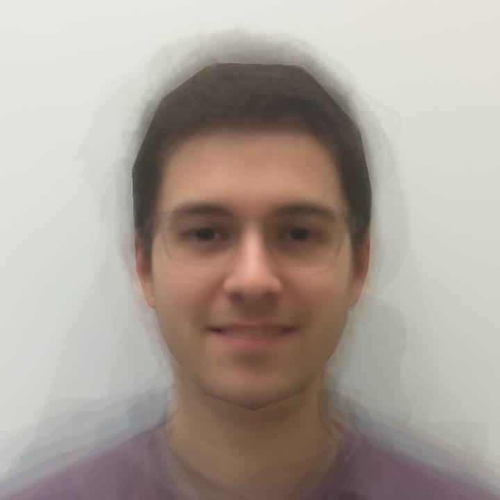
|
dlib-detector on our images lead to following results:
| average face shape from dlib | average class shape after morphing |
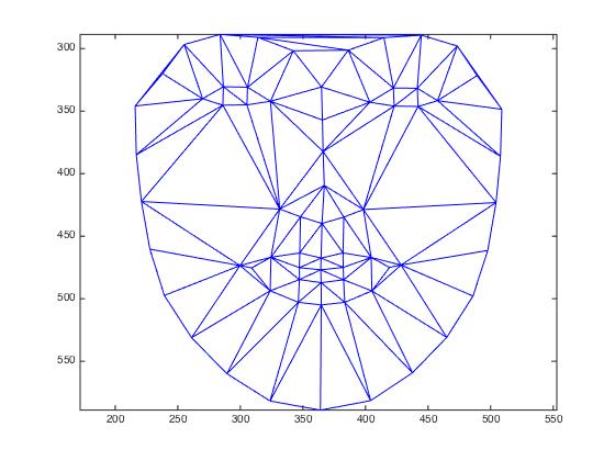
| 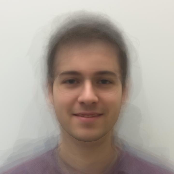
|
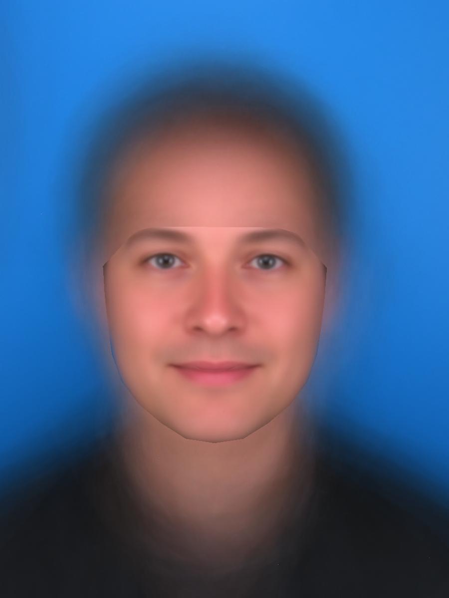
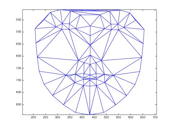
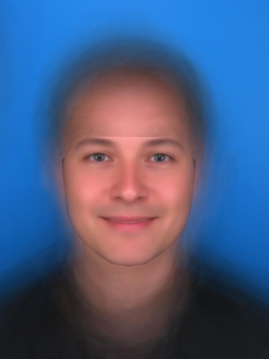
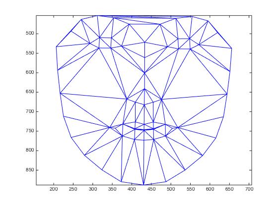
Utrecht data
| average face shape as detected by dlib | average shape from morphing |

| 
|
Discussion
Although the faces are not perfectly aligned within the images and might contain
asymmetries, the average face shapes are of symmetric shape. Plots of the average shapes (
triangulations) also reveals dlib to detect correspondences within the actual face only, while our points also
include the shape of the head. This results in a slightly different average face for the class
portraits compared to the result when using our points. When using our correspondences, the hairs are morphed as well and the intensity values
are explicitly sampled in the original images, while for the dlib-correspondences, this section of the
head is not morphed and the values there are derived from the background. As the faces are not
perfectly aligned, hair and background are mixed in the hair section.
This is also true for the Utrecht data set. All parts of the head outside the detected face are blurred.
Furthermore, a slight shortcoming of my implementation becomes visible here as the transition from face
to background is very distinct.
Bells and Whistles
As the Utrecht data set contains information on the expression of the person, i.e. whether the person
smiles or not, the average smiling and non-smiling face can be calculated. The approach is exactly the
same as depicted above, only difference regards the portraits based on which the average face is calculated.
Smiles A total number of 58 smiling faces was available, for which following average face shape and face could be retrieved:
| average face shape as detected by dlib | average shape from morphing |
| 
|
Non-Smiling A total number of 73 non-smiling faces was evaluated, for which following average face shape and face could be retrieved:
| average face shape as detected by dlib | average shape from morphing |
| 
|
Masculinization/Feminization
Methods
Utrecht data furthermore provides information on the gender of the faces. This information
can be used to calculate the average male and female face, respectively.
Furthermore, average male and female shape can be used to masculinize and feminize my portrait. To
do so, triangulation of my face was morphed into the mean shape of all men and women, respectively.
However, the problem was, that the Utrecht images have different sizes than my portrait
and scale of the faces are not equal to the one of my portrait.
Thus, I first brought Utrech images and my portrait to a width of 900px. In order to retrieve a comparable
scale, I slightly enlarged triangulation of the Utrecht data set. A third problem was a misalignment
between Utrecht triangulation and triangulation on my portrait. I thus shifted my portrait in order
to align it to the Utrecht data.
Results The mean male faces look as follows.
| average male face shape as detected by dlib | average shape from morphing |
| 
|
| average female face shape as detected by dlib | average shape from morphing |
| 
|
| my female face | my male face |
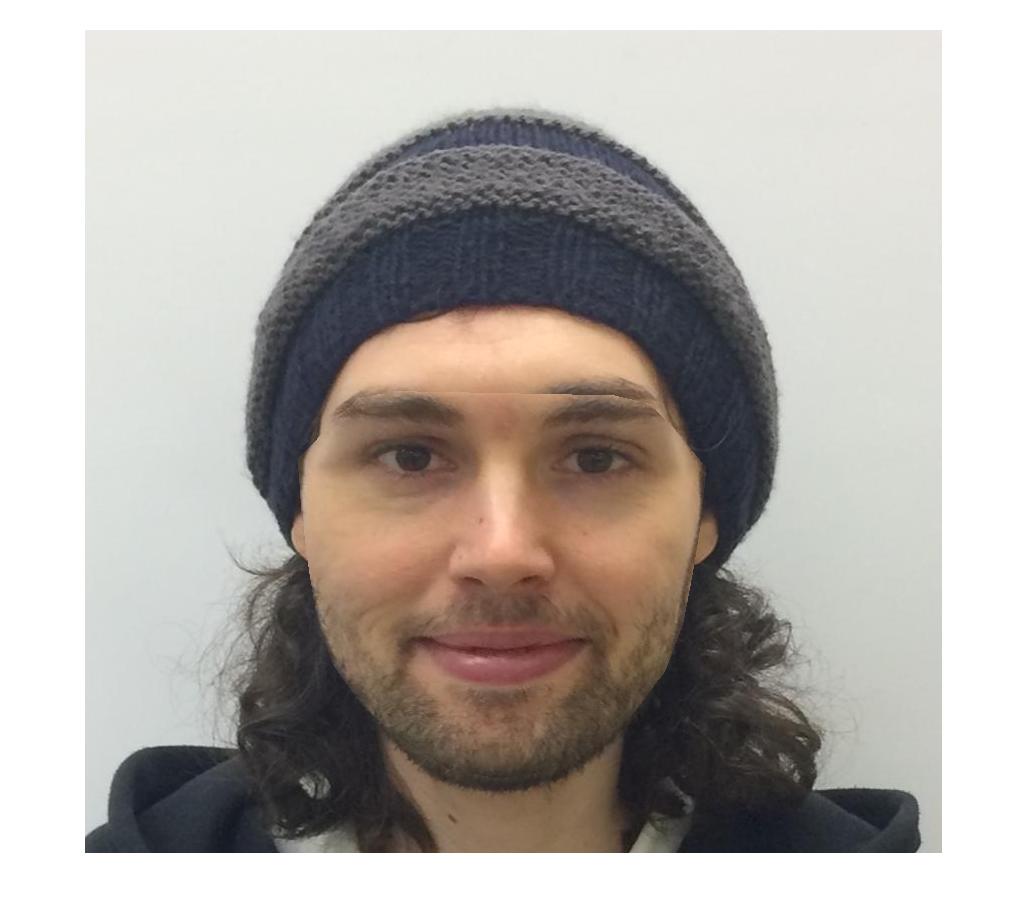
| 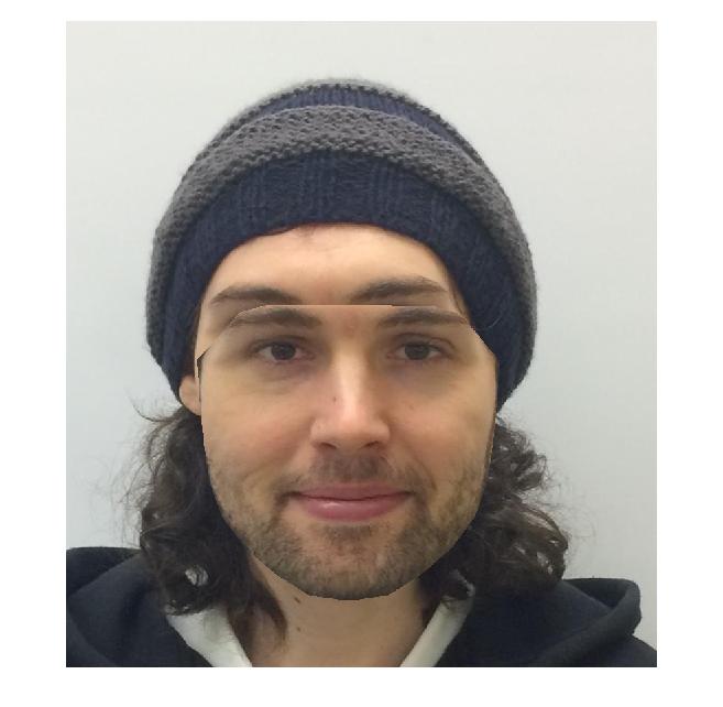
|
Discussion
The differences in facial characteristics between men and women are striking: The average female
face characteristics are much softer then the ones of men.
The problem is, that my face is not correctly located anymore. I ascribe this to a badly performed rescaling/
shifting step, which is described above and which was necessary as the images are of different
size. Furthermore, scales of faces in the Utrecht data set show variances. Thus,
despite I tried to align the images, I did anything wrong. For this reason, I was neither able
to overlay my face to the average Utrecht man/woman.