The goal of this assignment is to gradually morph one image until it is transformed into another one. In order to do that we can perform the following steps:
All these steps will be illustrated bellow together with the results.
mytsearch algorithm was used to locate the triangle to which every pixel in the image was attributed to. In parallel, the affine transformation that takes one triangle from the source image and transform it to its correspondent in the target image was calculated resulting in a 3x3 matrix. As indicated in the exercise definition I used the inverse transformation to get appropriate RGB color for all points.
warp_frac and dissolve_frac. For the warp_frac I just linearly increased its value from 0 to 1. For the dissolve_frac I chose a logarithmically spaced function (in MATLAB logspace) to go from 0 to 1 so that it takes a while to start integrating the target image into the final result.
In order to morph our faces I used the points provided by Carl and mine plus 10 points around the mouth in order to produce a better result. The only regions that remained badly alligned were the hair and the shoulder.

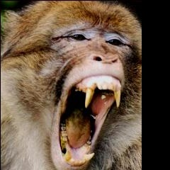
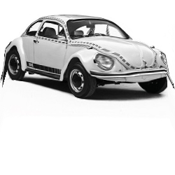
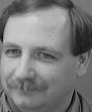
Source

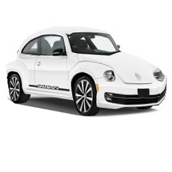
Target
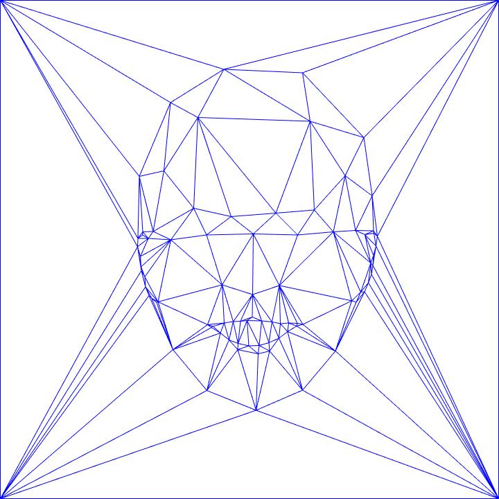
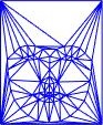
Average triangulation

Source "deformed" to target

Target "deformed" to source

Final morphing
This was a good result since the image are quite similar and the color transition was smooth enough to create a good result. The only bad deformation ocurred on the monkey teeths where I put some points but could not achieve the result I expected.

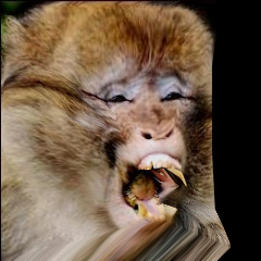
Source
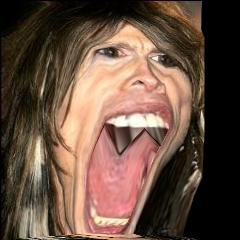
Target
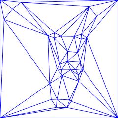
Average triangulation
Source "deformed" to target
Target "deformed" to source

Final morphing
This one did not give the result I expected. My guess is that since both objects are not in the same place in the image the affine transformation was too "strong" causing some undesired deformation on both images.
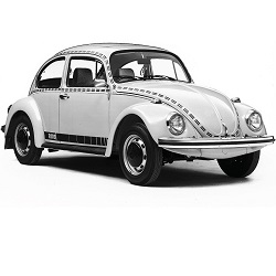
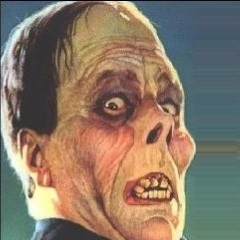
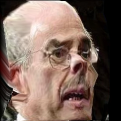
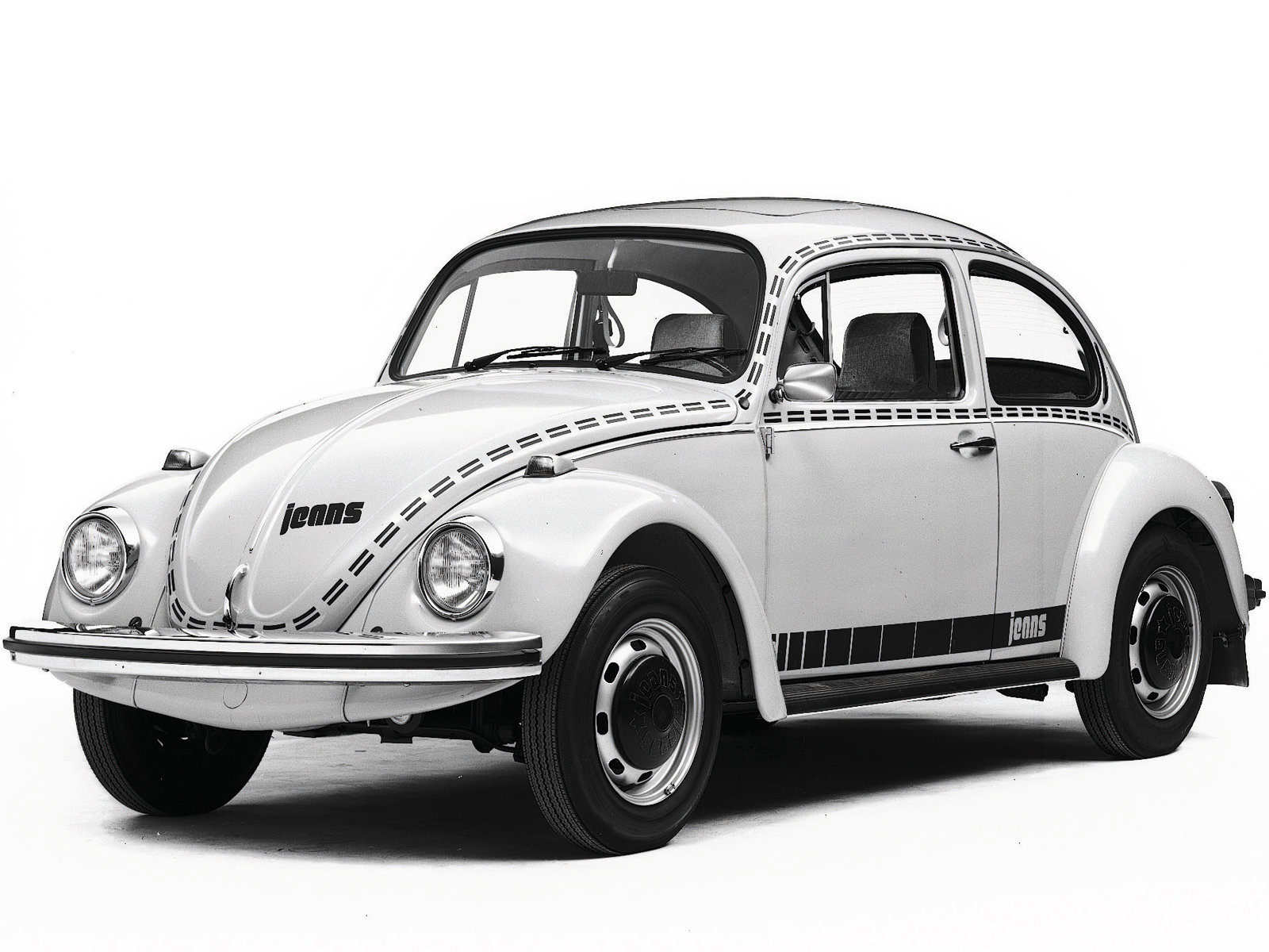
Source
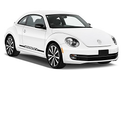
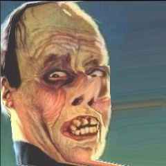
Target
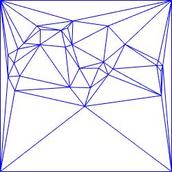
Average triangulation
Source "deformed" to target
Target "deformed" to source

Final morphing
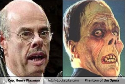
This one was another successful result since the comparison between Henry and this old version of the Phantom of the Opera was made by someone on the internet, even with very similar pictures! Therefore it was not hard to get the feature points and morph both images.

Source
Target
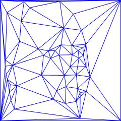
Average triangulation
Source "deformed" to target
Target "deformed" to source
Final morphing
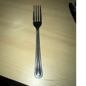
In this example I thought that creating many points between the fork tips would create a nice transition but the result was really bad. What worked better in the end was to use a smaller number of points at the upper region of the cutleries.
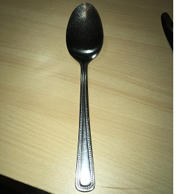
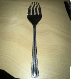
Source
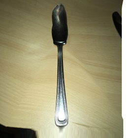
Target
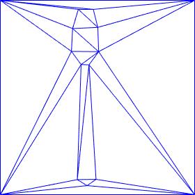
Average triangulation
Source "deformed" to target
Target "deformed" to source

Final morphing
In this example both objects have the same background and even similar silhouette. Therefore the result was good and a little amount of points were necessary to create the desired effect.
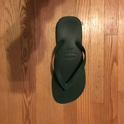
Source
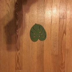
Target
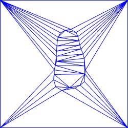
Average triangulation
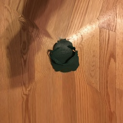
Source "deformed" to target
Target "deformed" to source
Final morphing
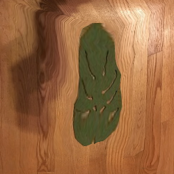
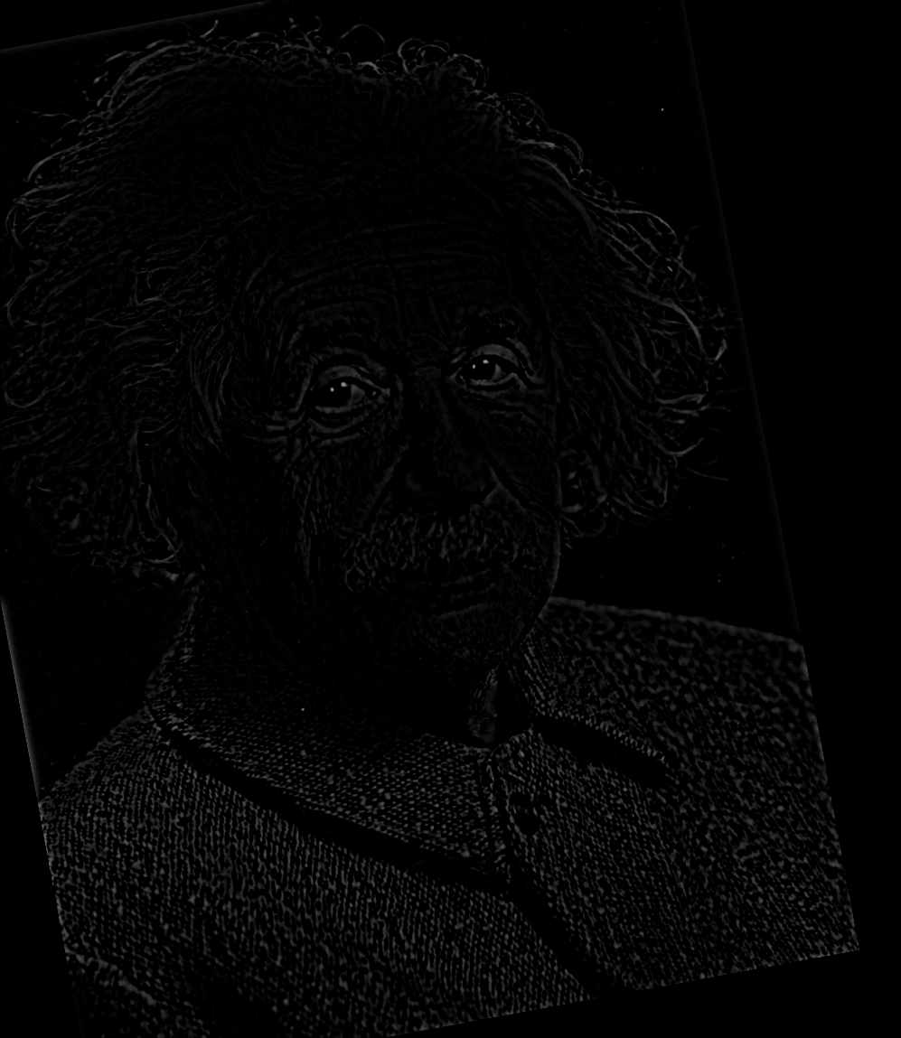
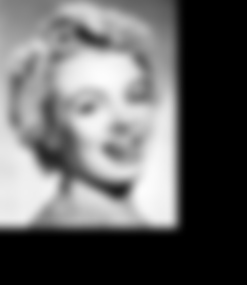
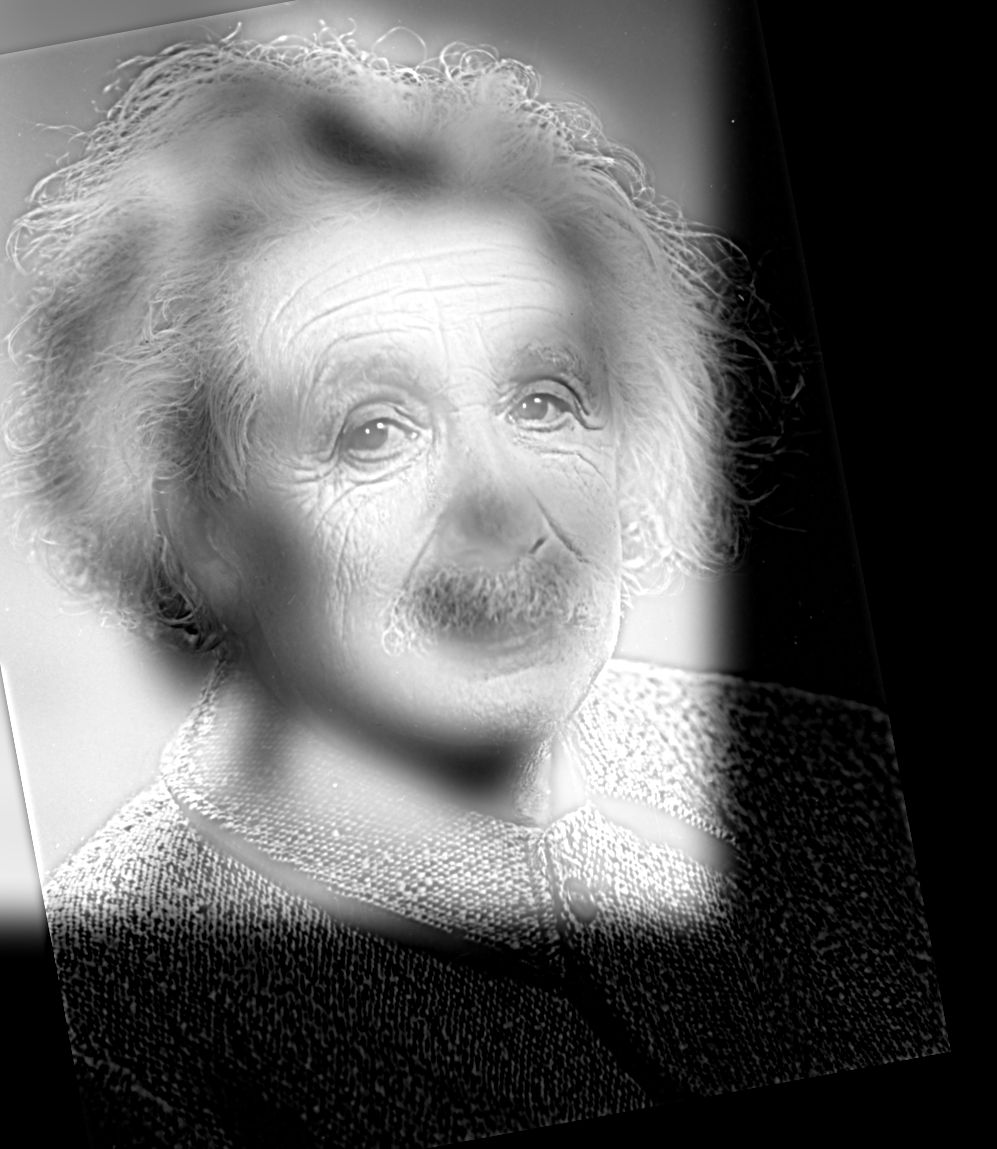
Here I morphed the high pass filtered photo of Albert Einstein with the low pass filtered photo of Marilyn Monroe. Curiously the result in my opinion is worse than the original one and I believe this is because now both Albert and Marilyn are brought to a common image. In this case it is hard to spot Einstein from the high frequences and Monroe from the low frequences because they represent deformed versions of their original pictures.
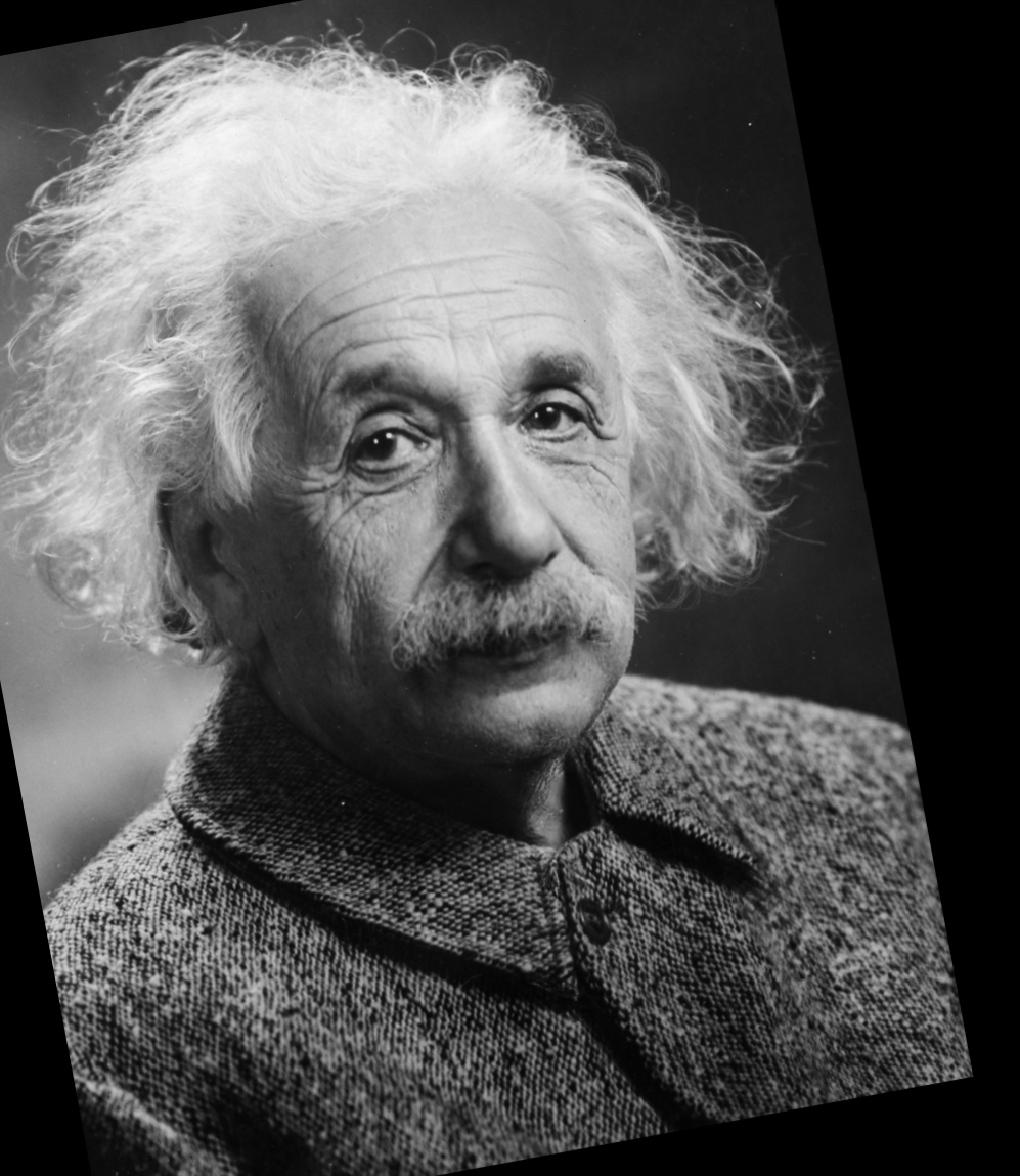
Source
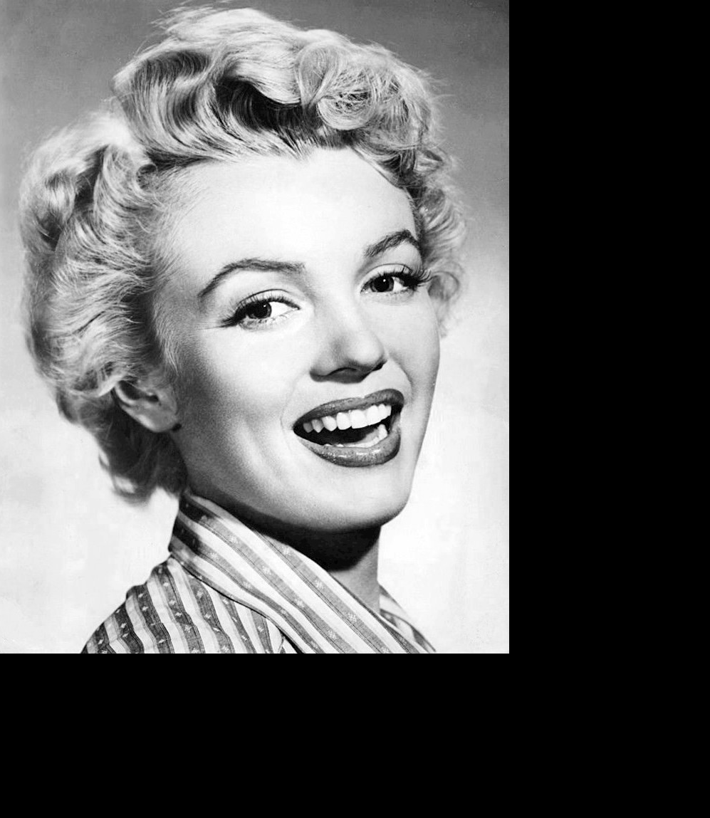
Target
Average triangulation
Source "deformed" to target
Target "deformed" to source
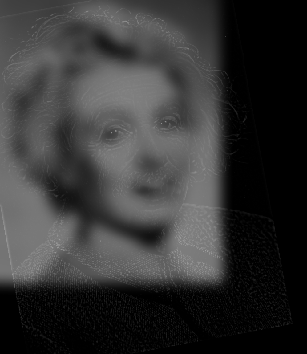
Final morphing
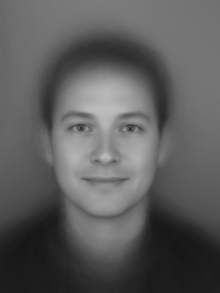
In this part of the assignment the goal is to find "mean faces" of datasets. By doing this we can also find a feminine face and male face and perform nice combinations!
The result for the average class face using the points generated by the students was pretty bad. Probably the point location was not accurate enough and as a result the standard deviation between the points was high.
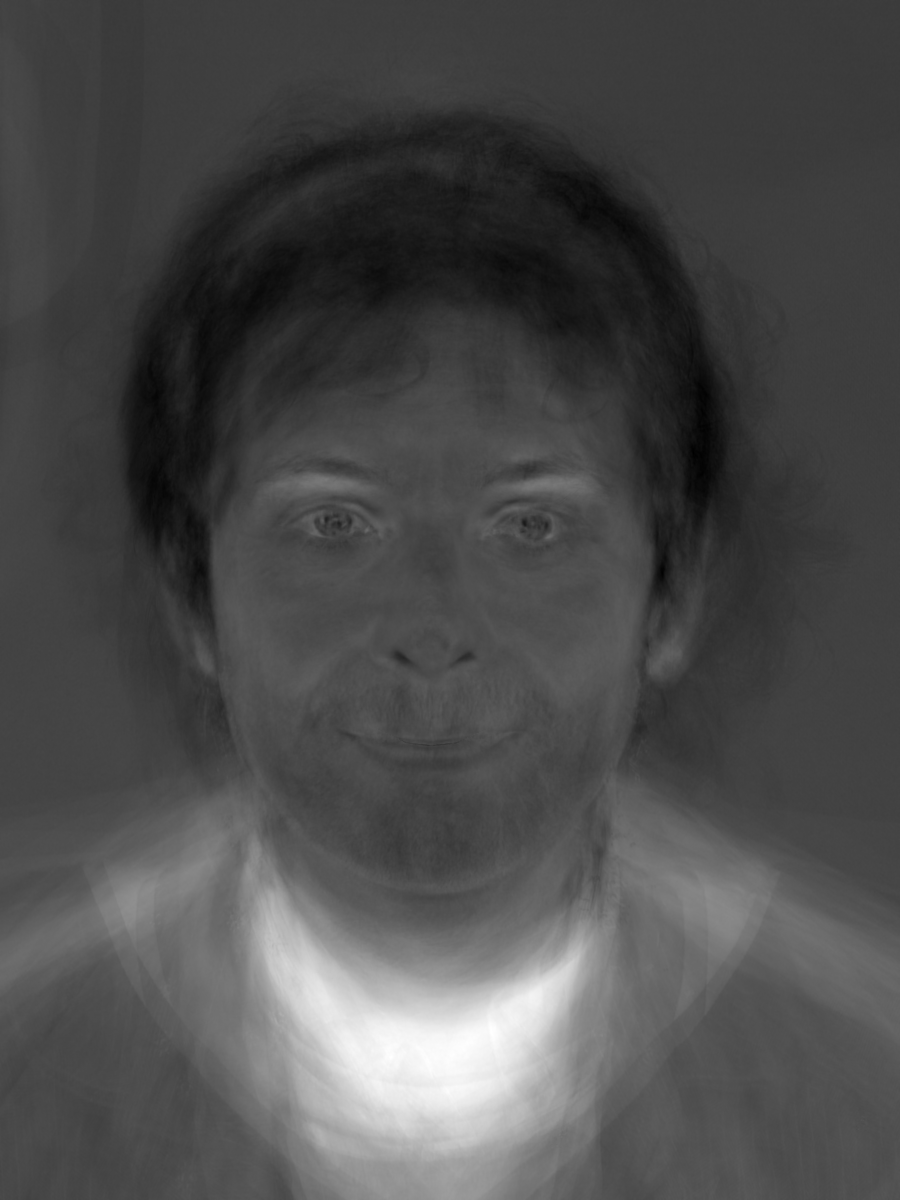
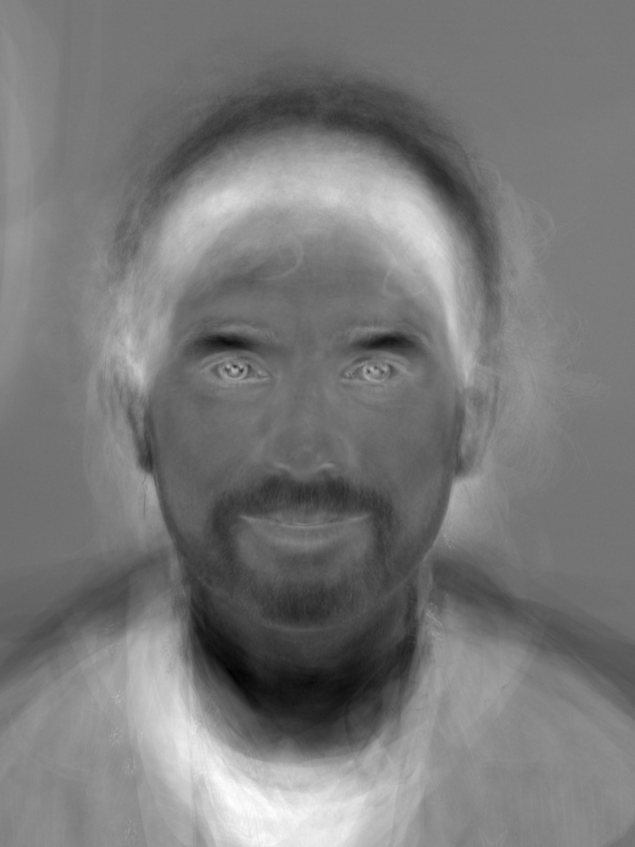
On the other hand the result generated by the algorithm was much better! We can clearly see a face in there, and a male one since the class was mainly composed by men.
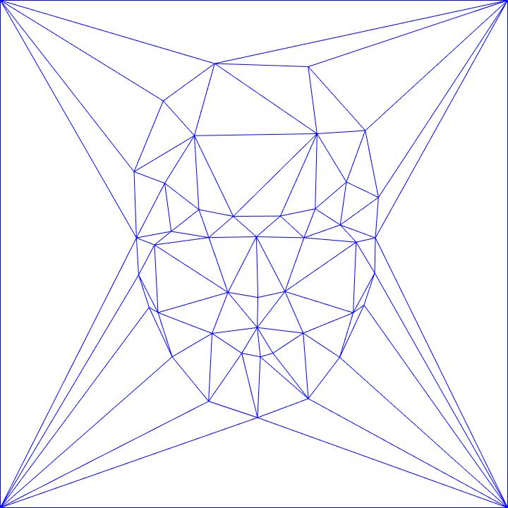
Average shape using points generated by the students.
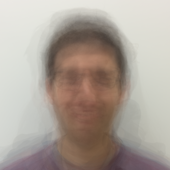
Mean face using points generated by the students.
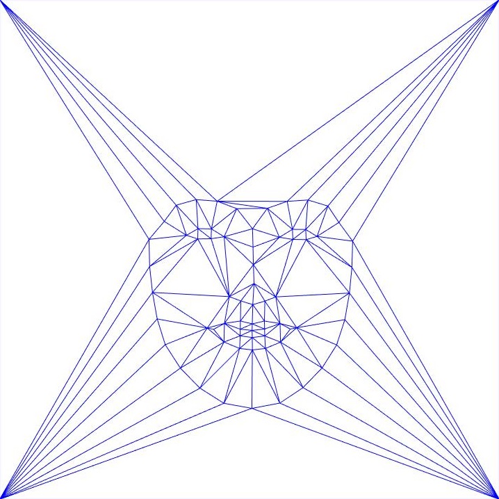
Average shape using points generated by the algorithm.
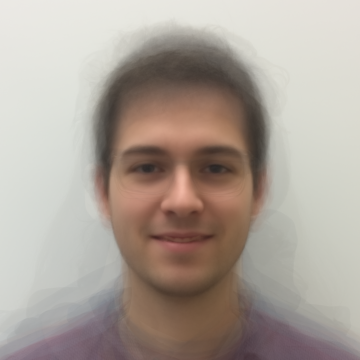
Mean face using points generated by the algorithm.
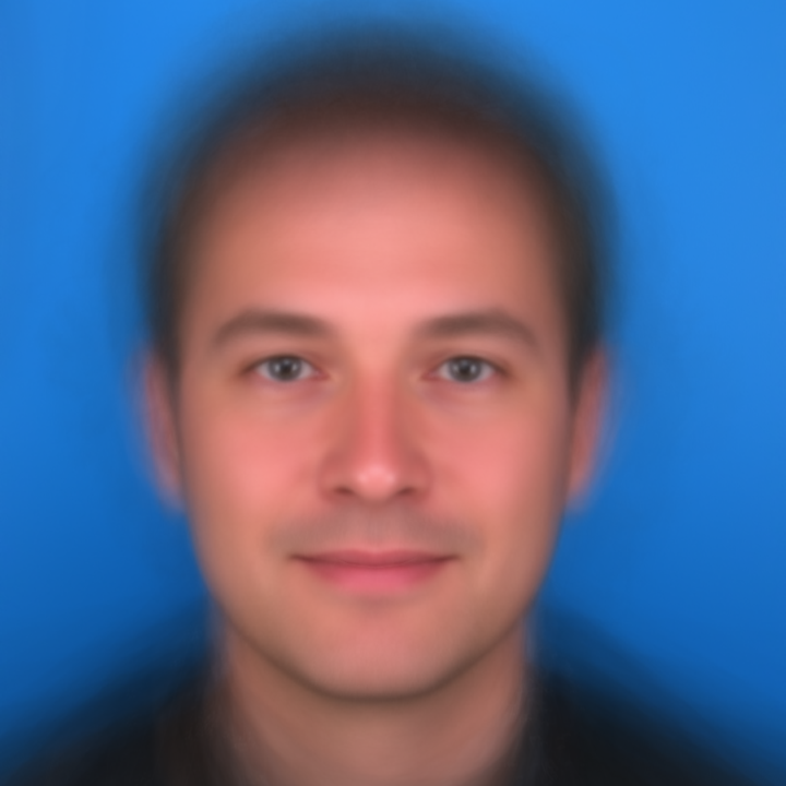
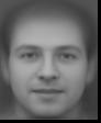
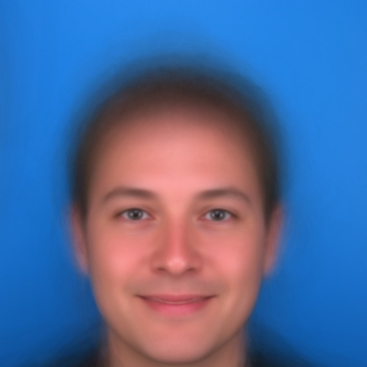
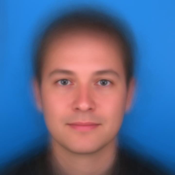
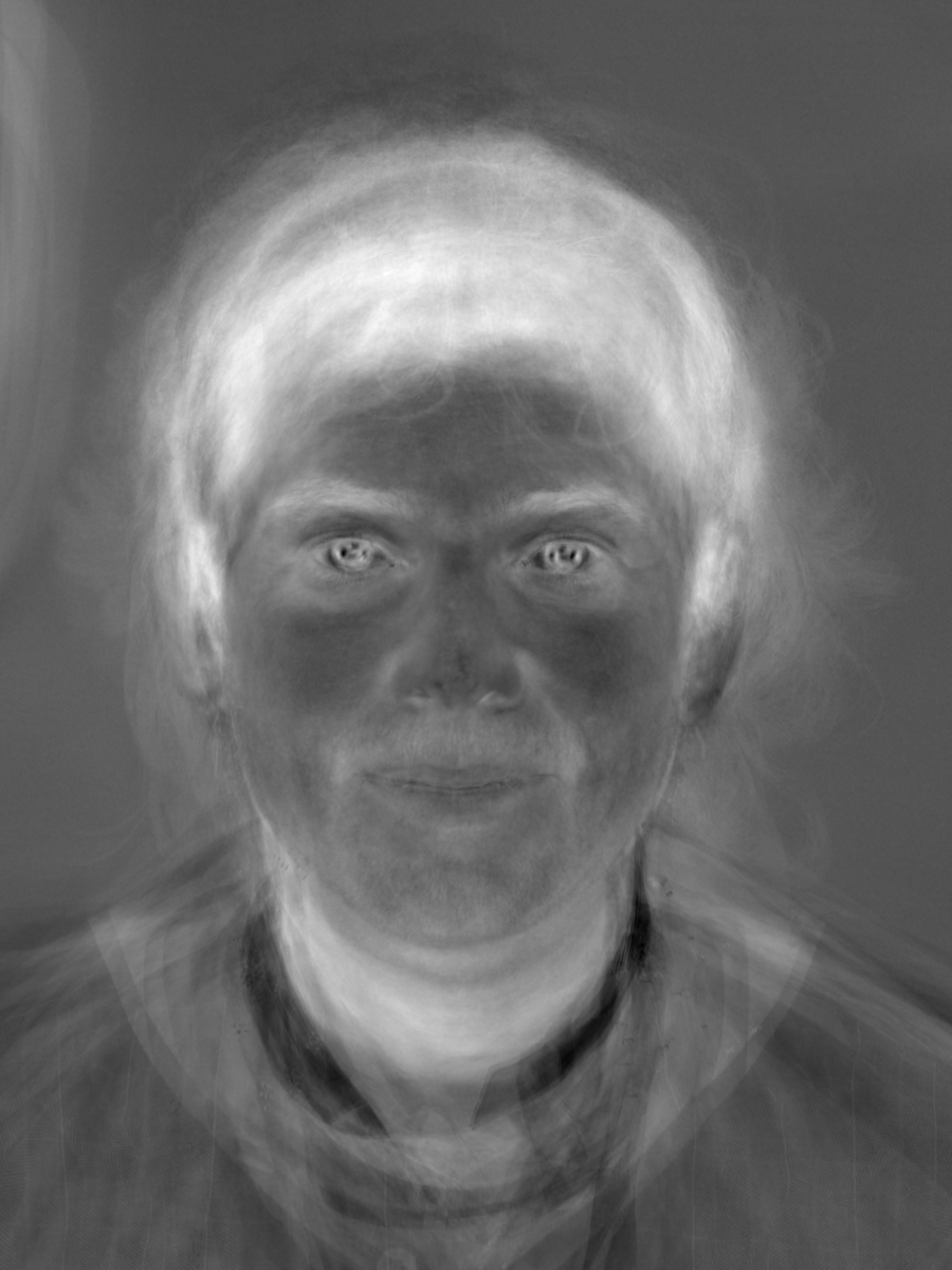
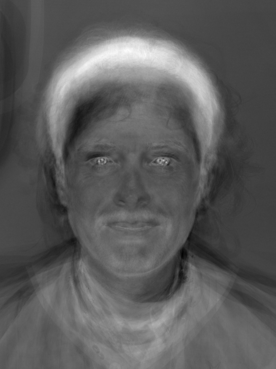
For the Utrecht database we were asked to use the algorithm that detects points automatically. It generates 68 points around the face and ignores the hair. It generated a clear face probably because we used a lot of different pictures.
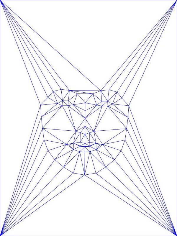
Average shape of the Utrecht database.
Mean face of the Utrecht database.
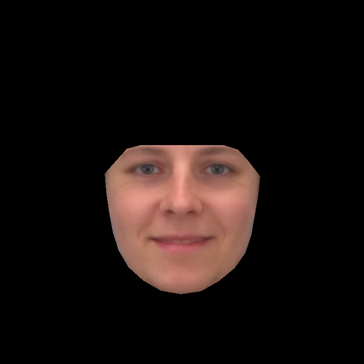
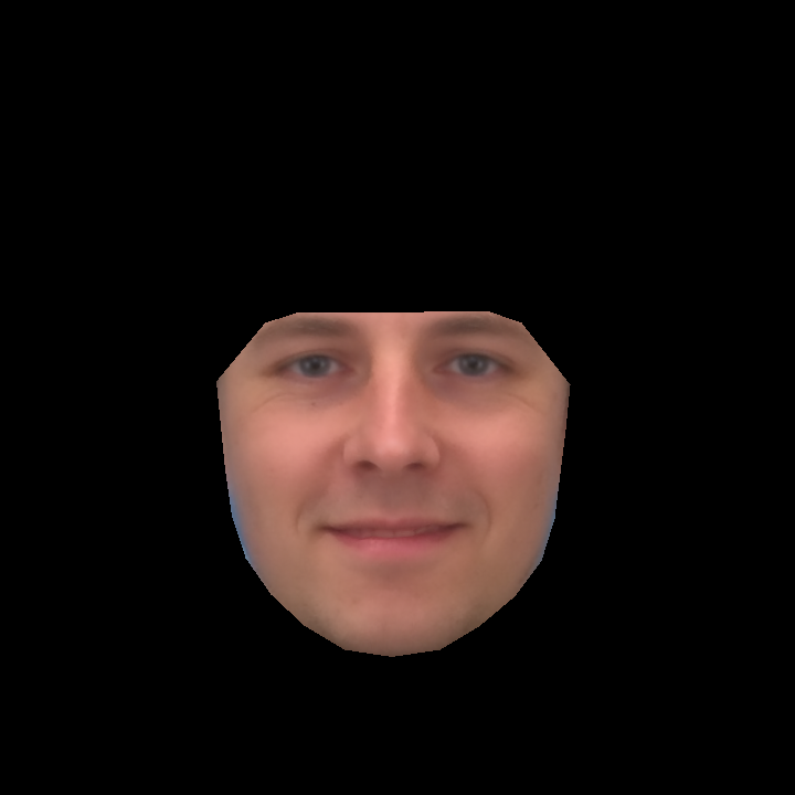
In this part the idea is to morph my own image with the average of the men and the average of the women. Since the difference in the hair is too visible I decidec to crop it out for a more clear result. The difference between my feminine face, my masculine face and original face are quite visible! The feminine face tends to have more round shapes and the masculin more straight shapes, and also the masculine has a bigger nose than the feminine one. Another thing I found interesting is that the average masculine face was almost identic to the avereage face of the whole database!
Average feminin face.
Morph between my face (50%) and the average feminine face (50%).
Average masculin face.
Morph between my face (50%) and the average masculine face (50%).
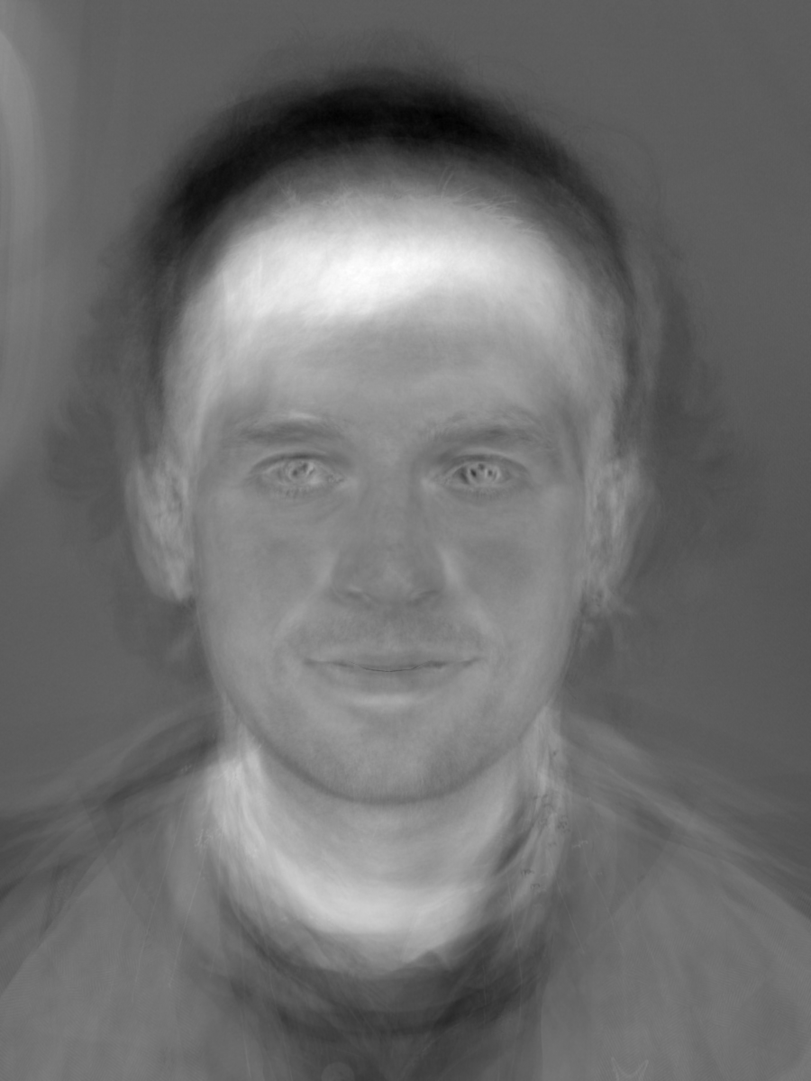
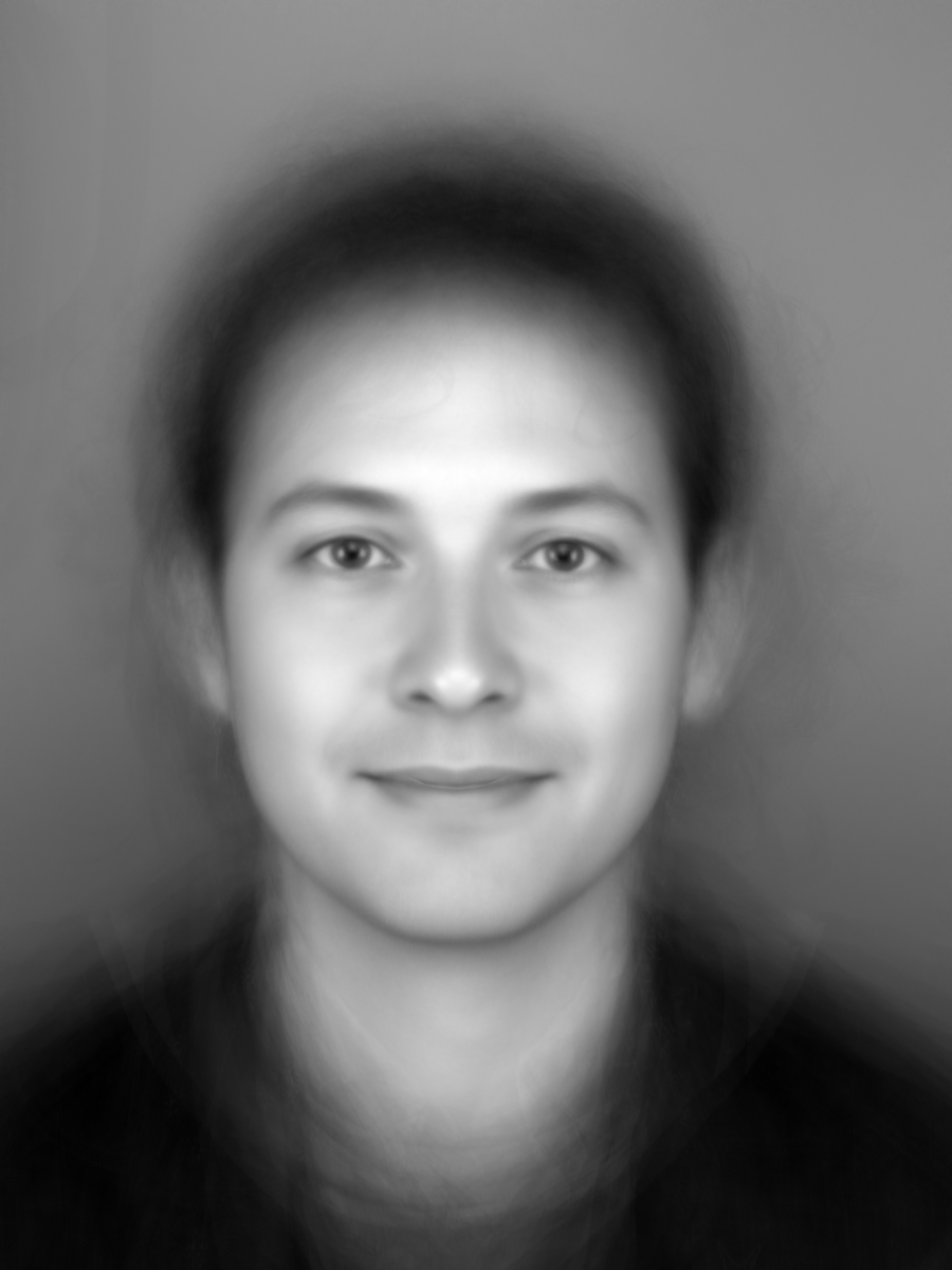
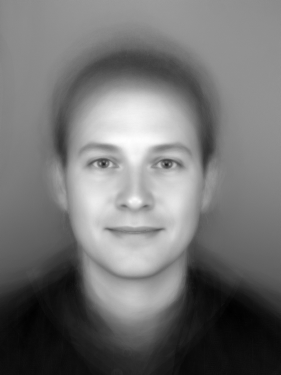
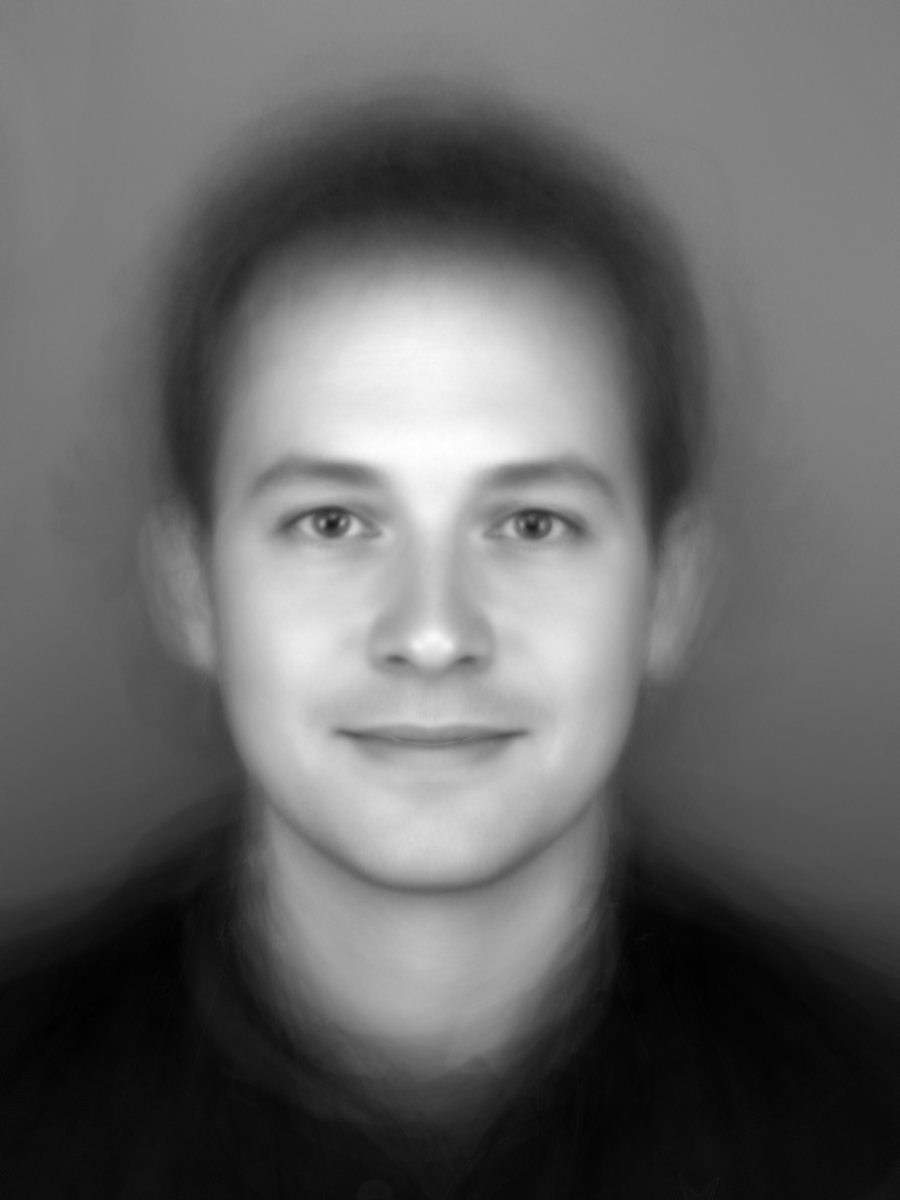
Just to check if the average face would differ that much by using a specific database, I tested on another dataset. This one has 10 pictures of 40 different people. The automatic feature points algorithm could recognize 390 out of 400 pictures. The average face differs a little bit from the Utrecht database but still keeps a similar shape.
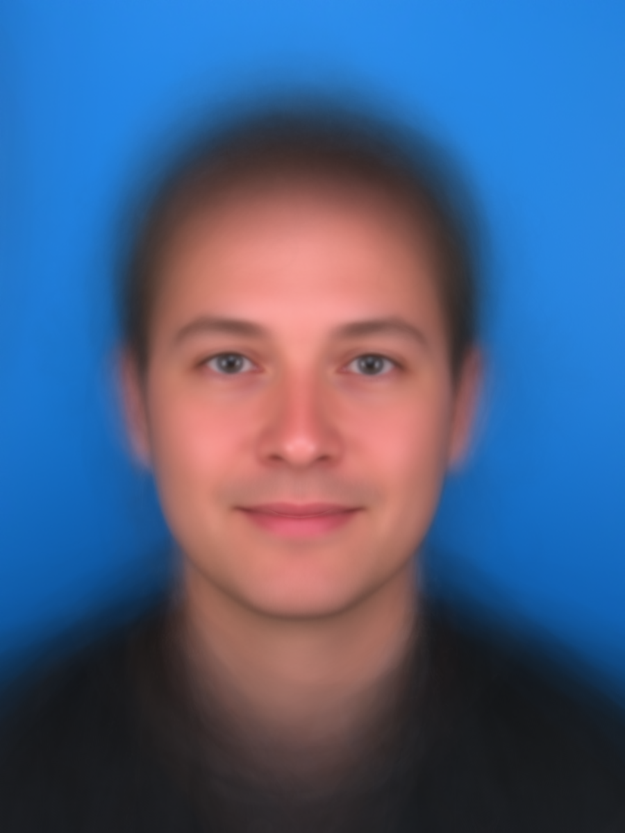
Face of a man on the dataset.

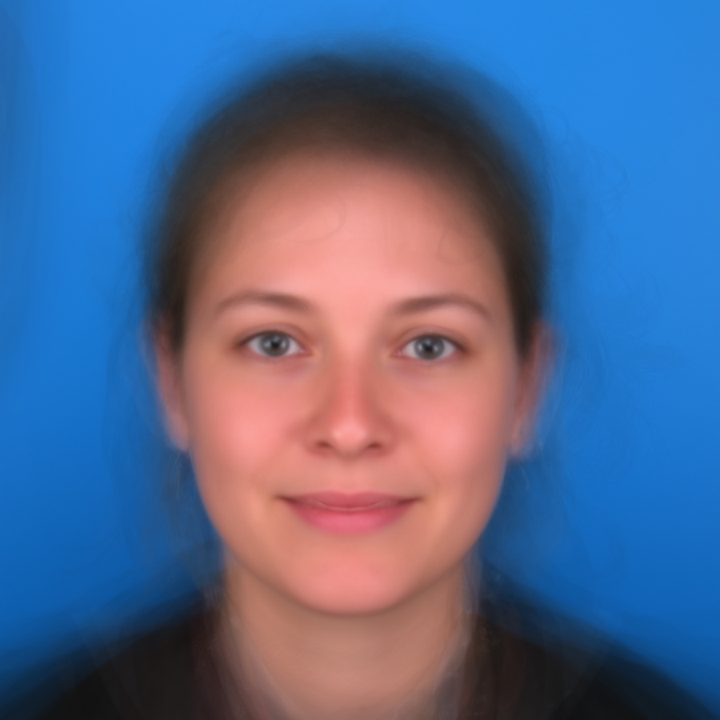
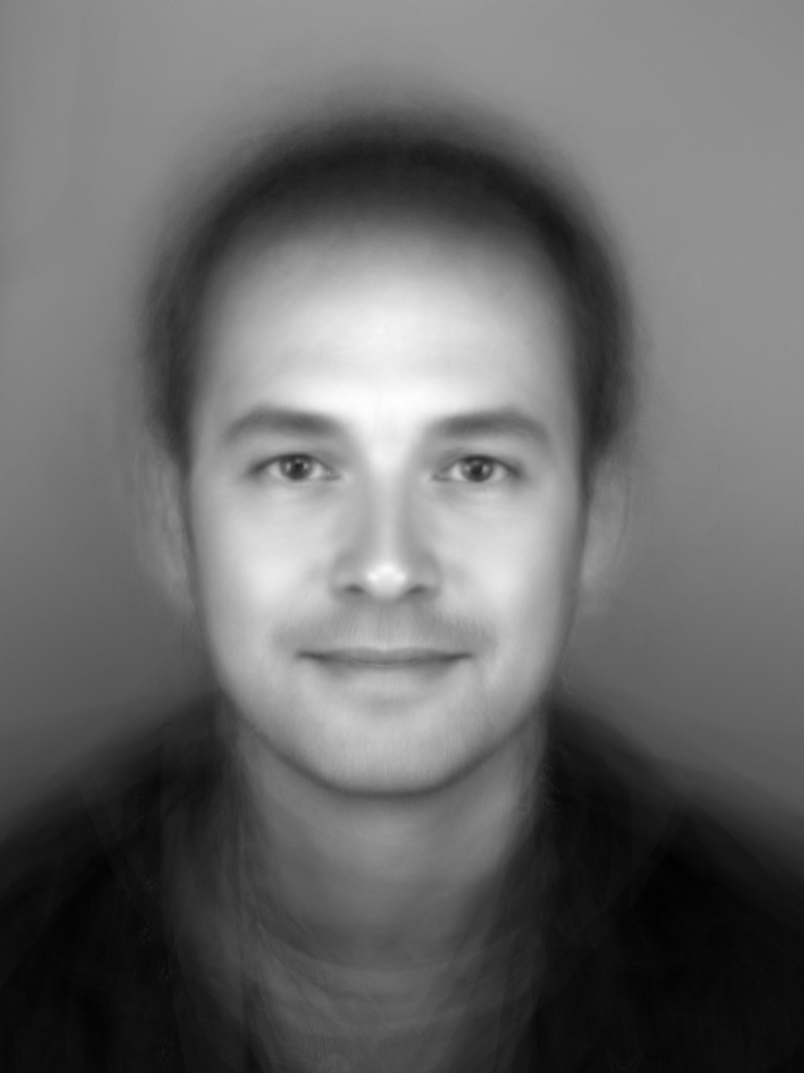
Face of a woman on the dataset.
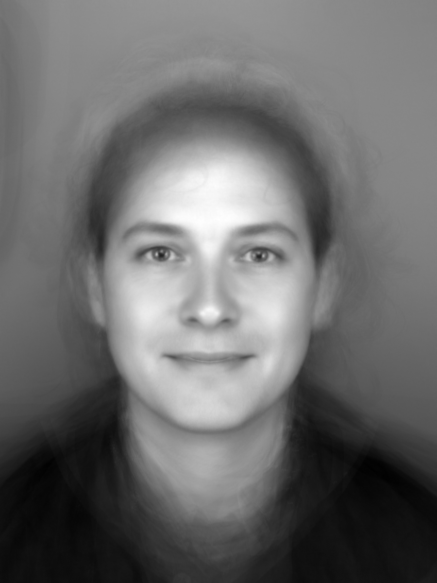
Average shape of the dataset.
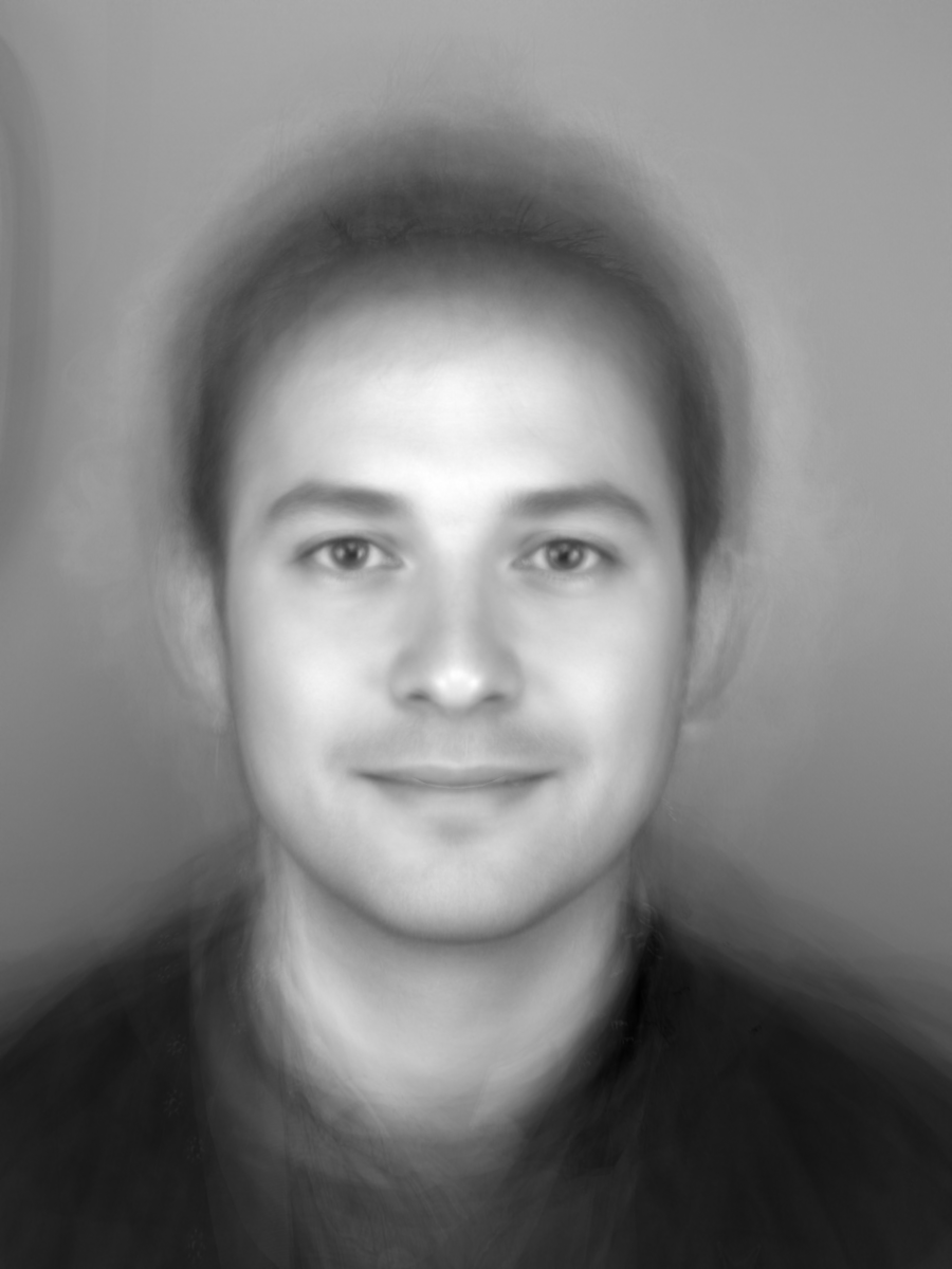
Mean face of the database.
Average smile face.
My face being forced to smile.
Average serious face.

My face being forced to be serious.
Mean face.
Eigenface 1.
Eigenface 2.
Eigenface 3.
Eigenface 4.
Eigenface 5.
Mean face with eigenface 1.
Mean face with eigenface 2.
Mean face with eigenface 3.
Mean face with eigenface 4.
Mean face with eigenface 5.
Mean face with eigenface 6.