


As the pictures in the first approach are small, one can apply the shift detection directly on the original image. This resulted in following detected shifts:
The detected shifts| Image | dx Green (SSD) | dy Green (SSD) | dx Blue (SSD) | dy Blue (SSD) | dx Green (CCR) | dy Green (CCR) | dx Blue (CCR) | dy Blue (CCR) | 00106v.jpg | 2 | -5 | -13 | 7 | -2 | -5 | 1 | -10 |
| 00757v.jpg | -2 | -3 | -5 | -5 | -2 | -3 | -5 | -5 |
| 00888v.jpg | 0 | -7 | -1 | -12 | 0 | -7 | -1 | -12 |
| 00889v.jpg | -1 | -3 | -3 | -4 | -1 | -3 | -3 | -4 |
| 00907v.jpg | 1 | -3 | 0 | -6 | 1 | -3 | 1 | -6 |
| 00911v.jpg | 1 | -12 | 1 | -13 | 1 | -12 | 1 | -13 |
| 01031v.jpg | 0 | -3 | -1 | -4 | 0 | -3 | -1 | -4 |
| 01657v.jpg | 0 | -6 | -1 | -12 | 0 | -6 | -1 | -12 |
| 01880v.jpg | -2 | -8 | -4 | -14 | -2 | -8 | -4 | -14 |
As the table shows, both approaches for shift detection lead to very similarly good results for most images. The largest differences occur for 00106v.jpg. The shift for this image
was not well detected by neither of the approaches, based on a visual control.
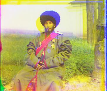
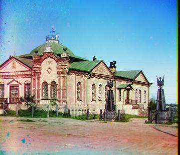
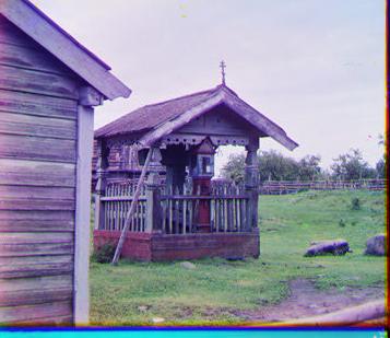
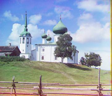
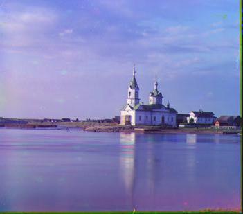
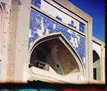
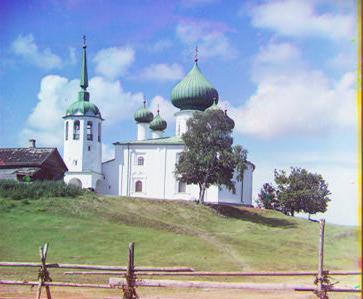
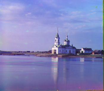
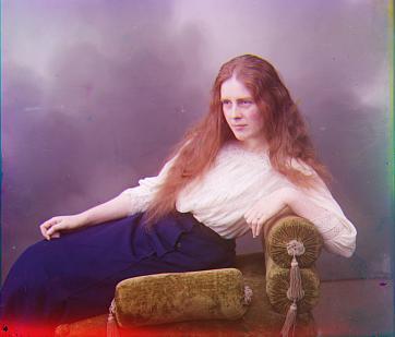
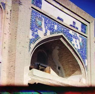
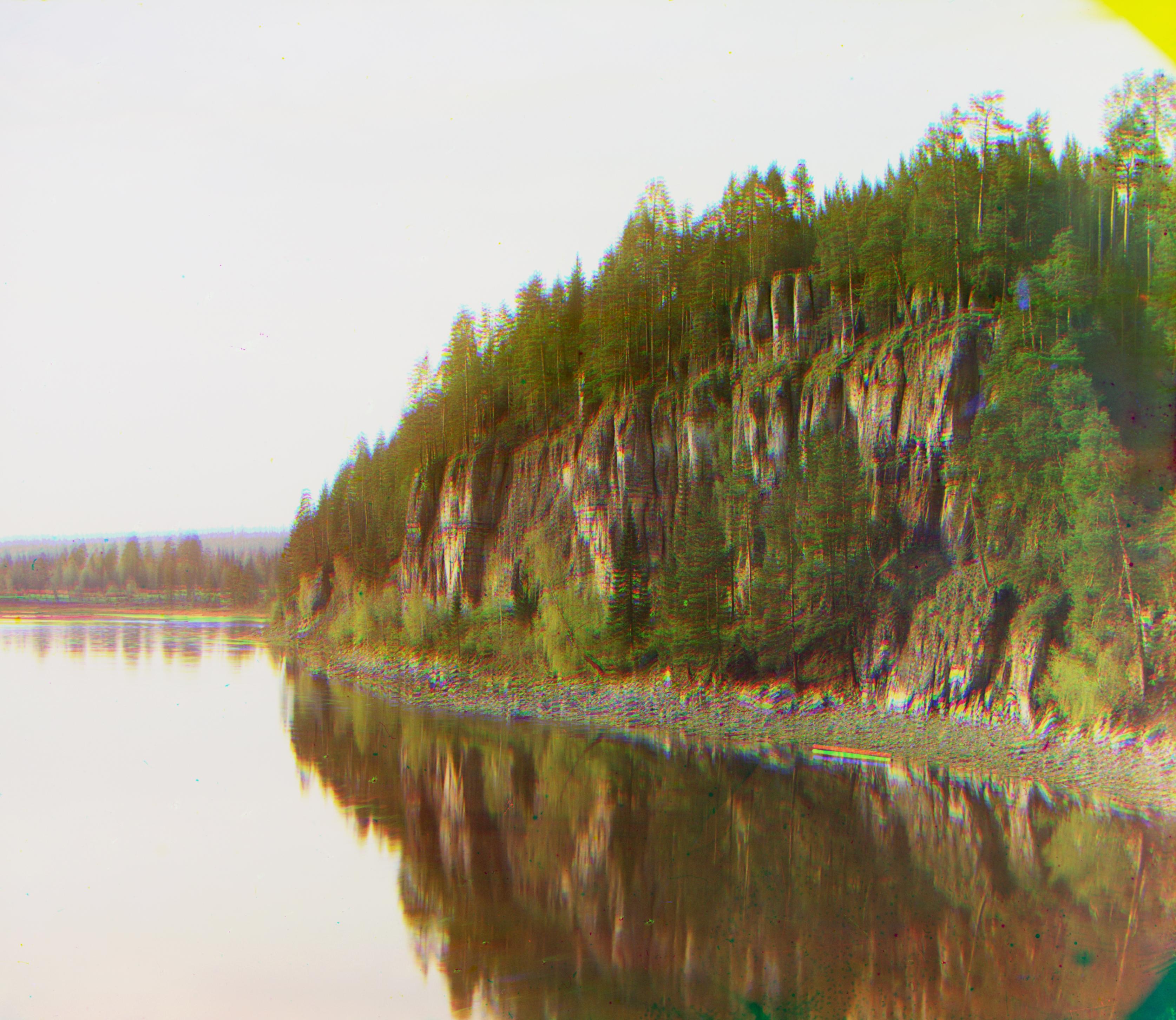
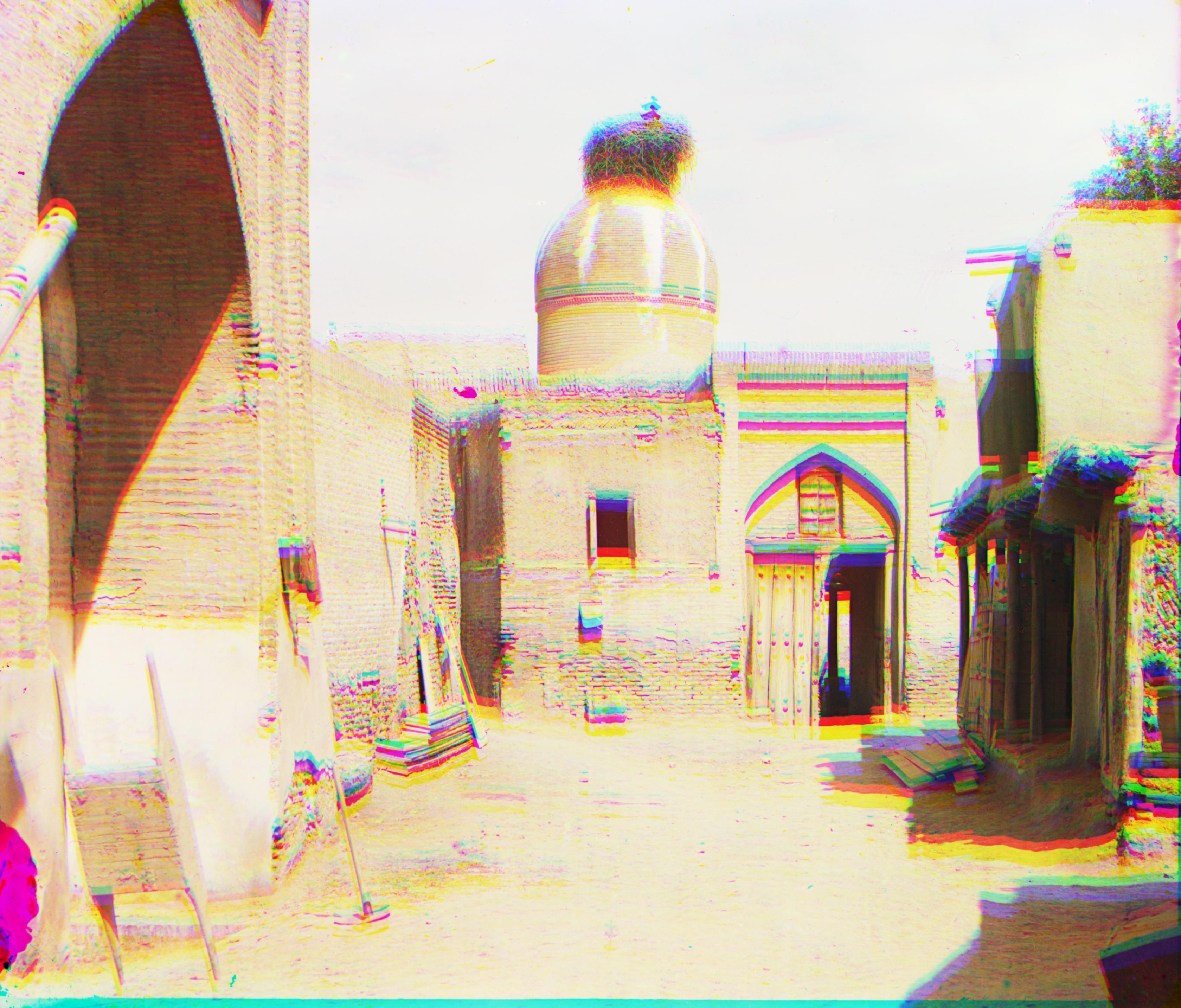
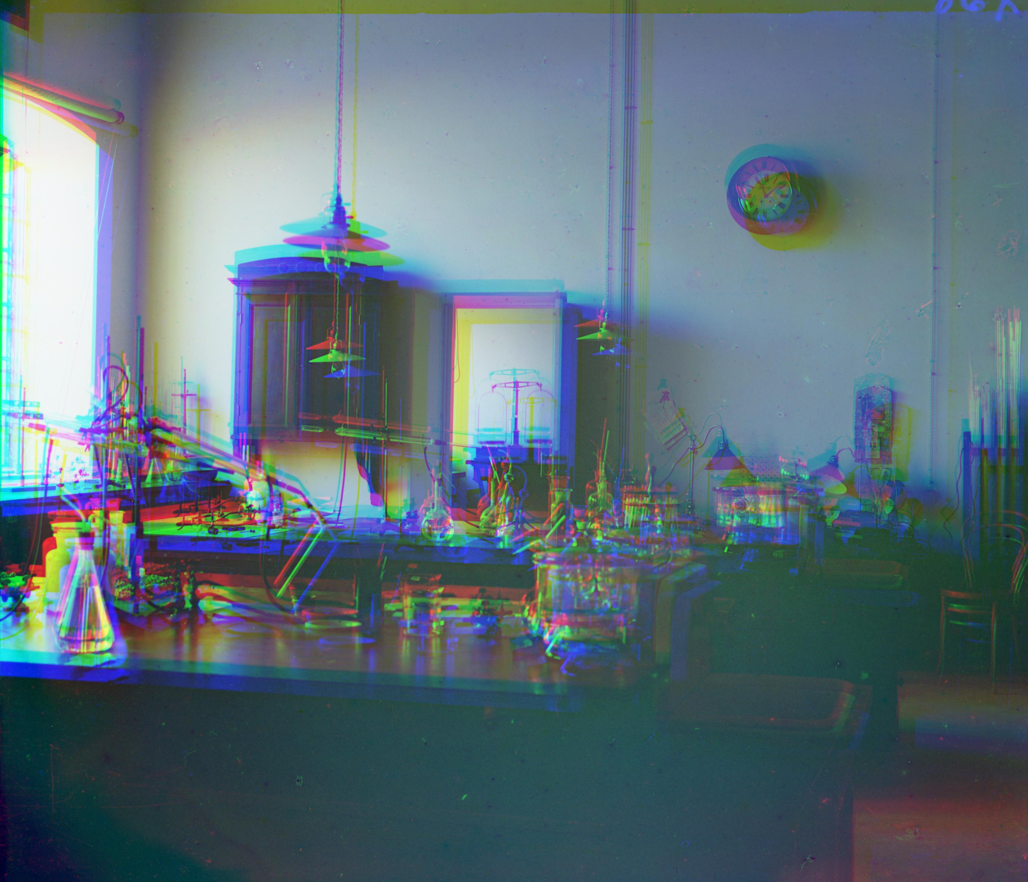
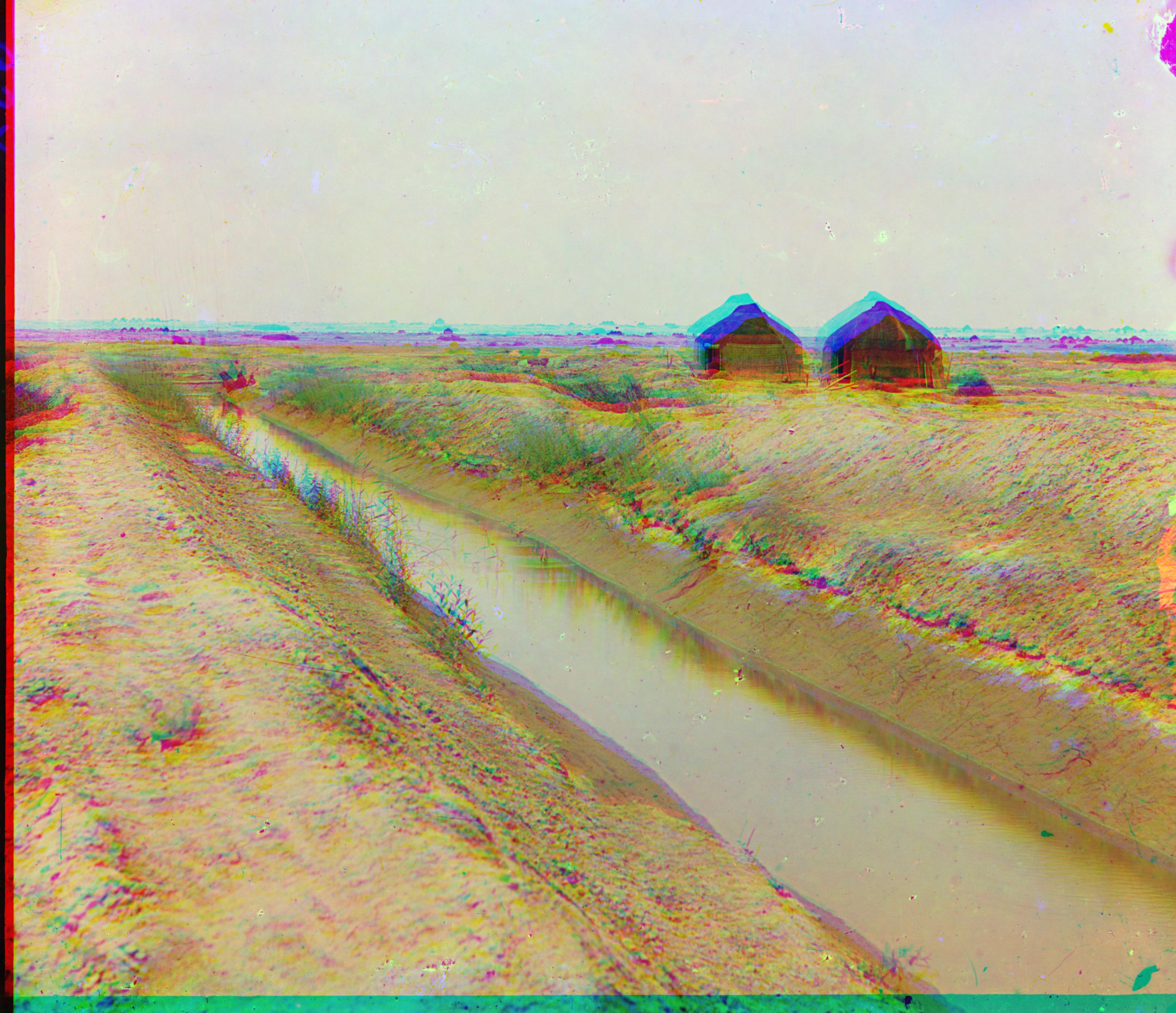
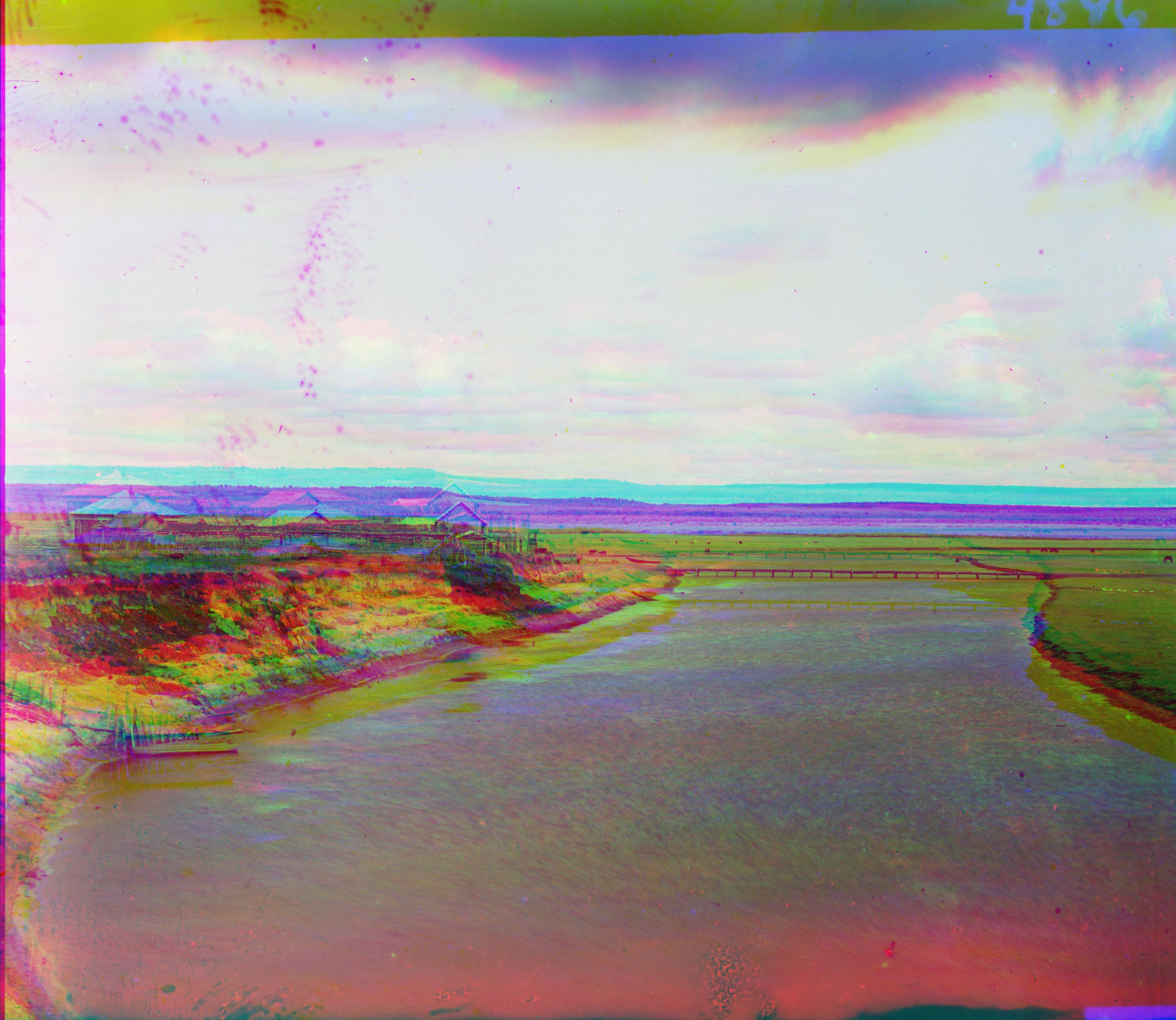
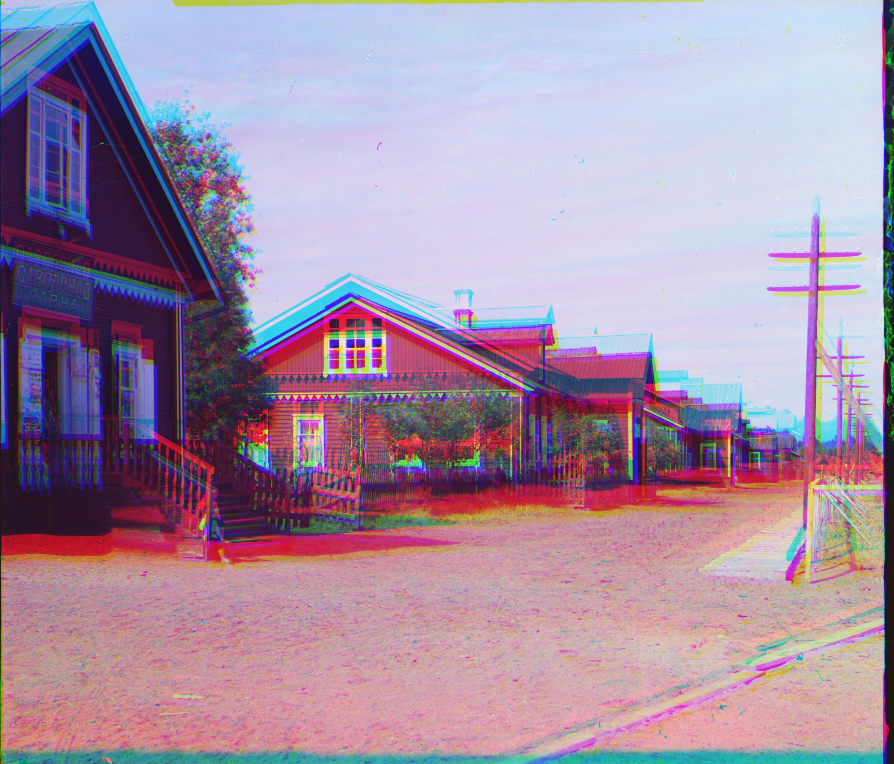
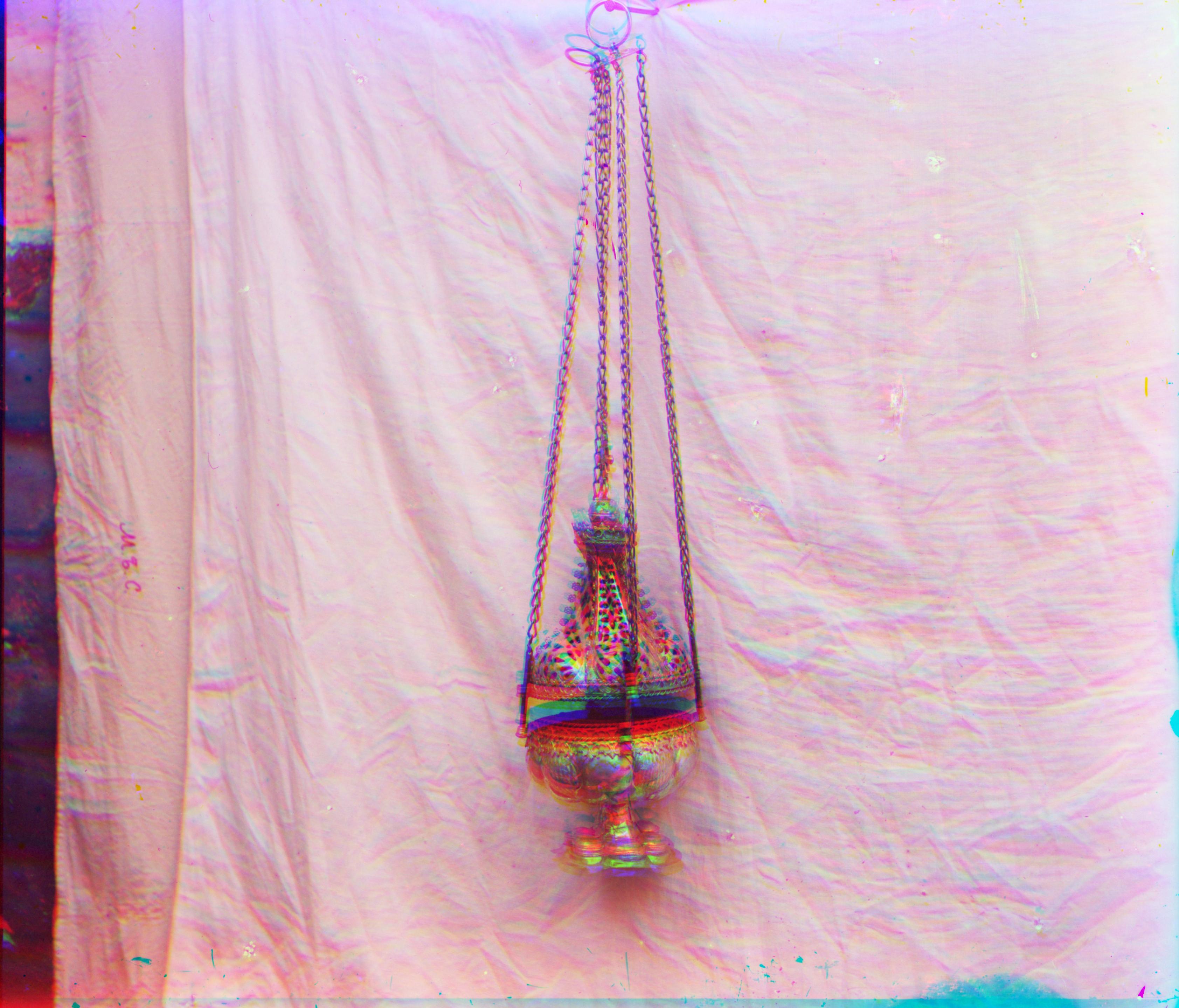
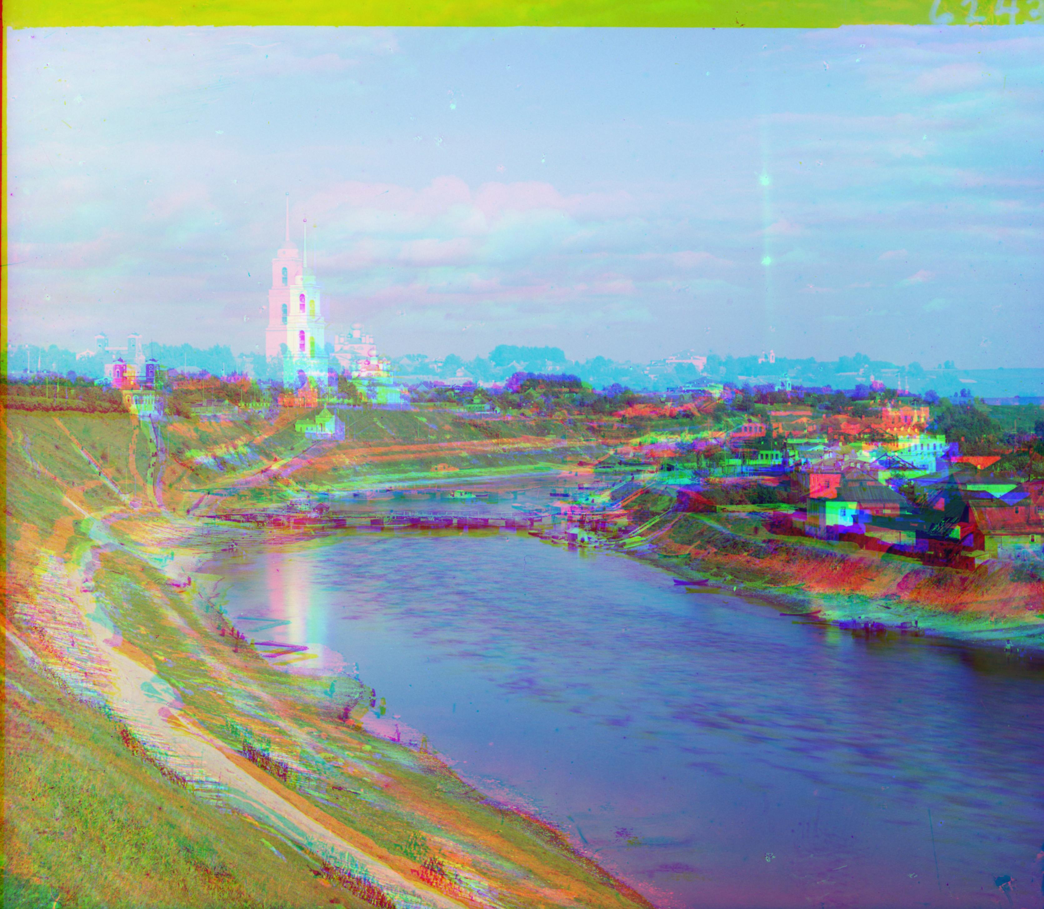
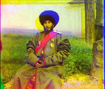
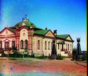
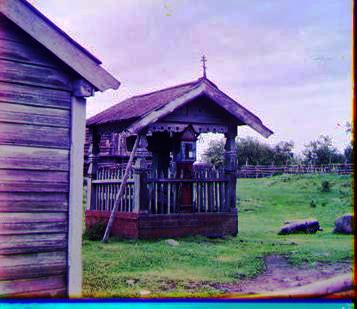
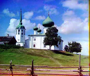
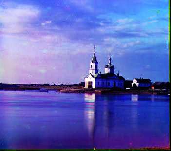
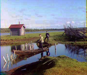
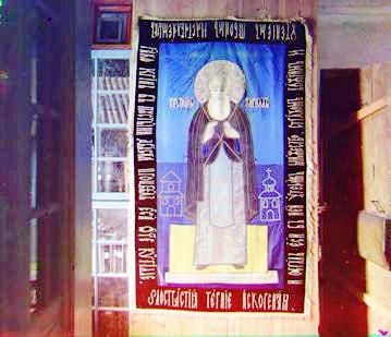
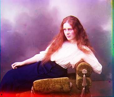
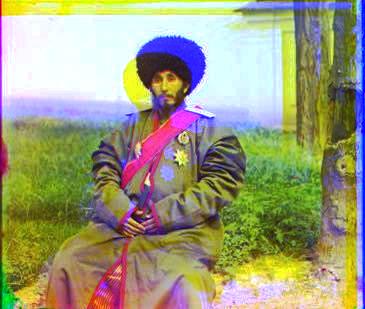
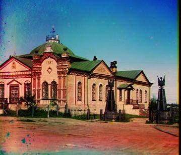
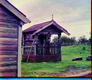
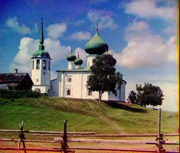
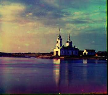
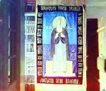
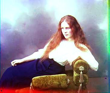
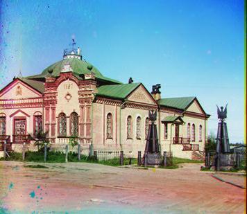
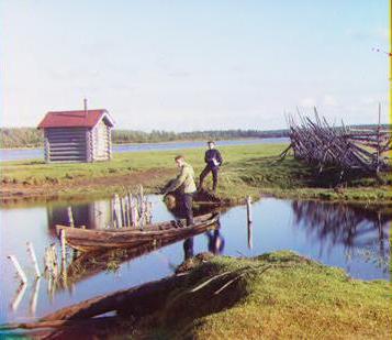
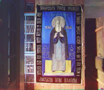
The following pictures show the corrections from the SSD:
|
|
|
|
| 00106v.jpg | 00757v.jpg | 00888v.jpg | 00889v.jpg |
|
|
|
|
| 000907v.jpg | 00911v.jpg | 01657v.jpg | 00889v.jpg |
|
| |||
| 01880v.jpg |
And this are the results from the CCR-based shift-estimation:
| 
| 
| 
| 00106v.jpg | 00757v.jpg | 00888v.jpg | 00889v.jpg |
| 
| 
| 
| 000907v.jpg | 00911v.jpg | 01657v.jpg | 00889v.jpg |
| |||
| 01880v.jpg |
| 
| 
| 
| 00029u.tif | 00087u.tif | 00128u.tif | 00458u.jpg |
| 
| 
| 
| 00737u.tif | 00822u.tif | 00892u.tif | 01043u.tif |
| |||
| 01047u.tif |
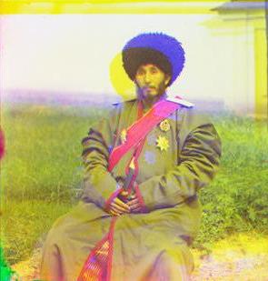
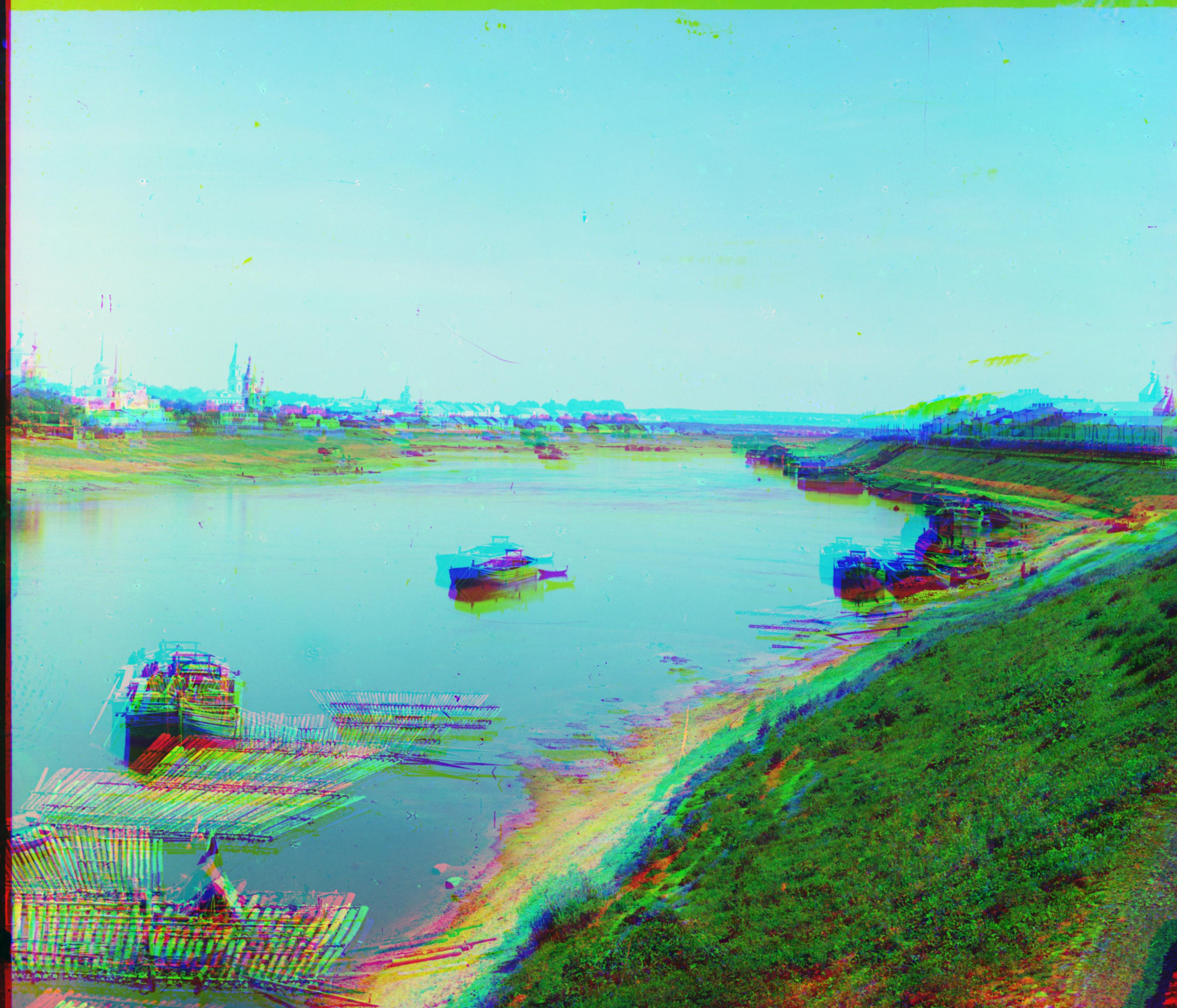
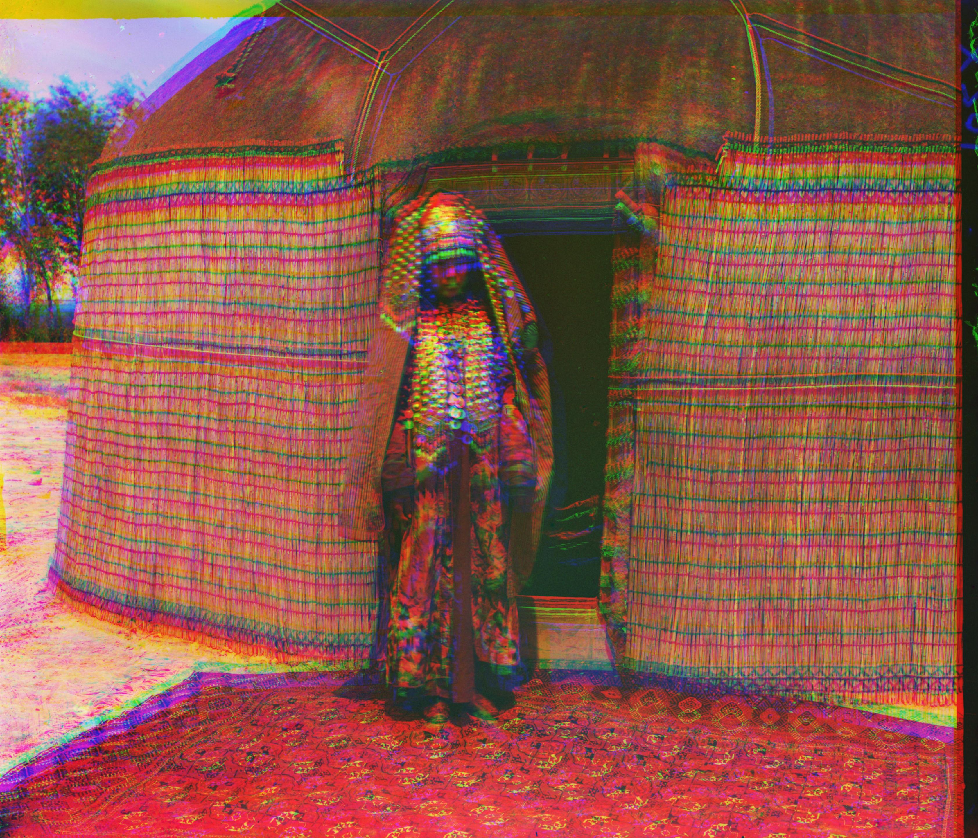
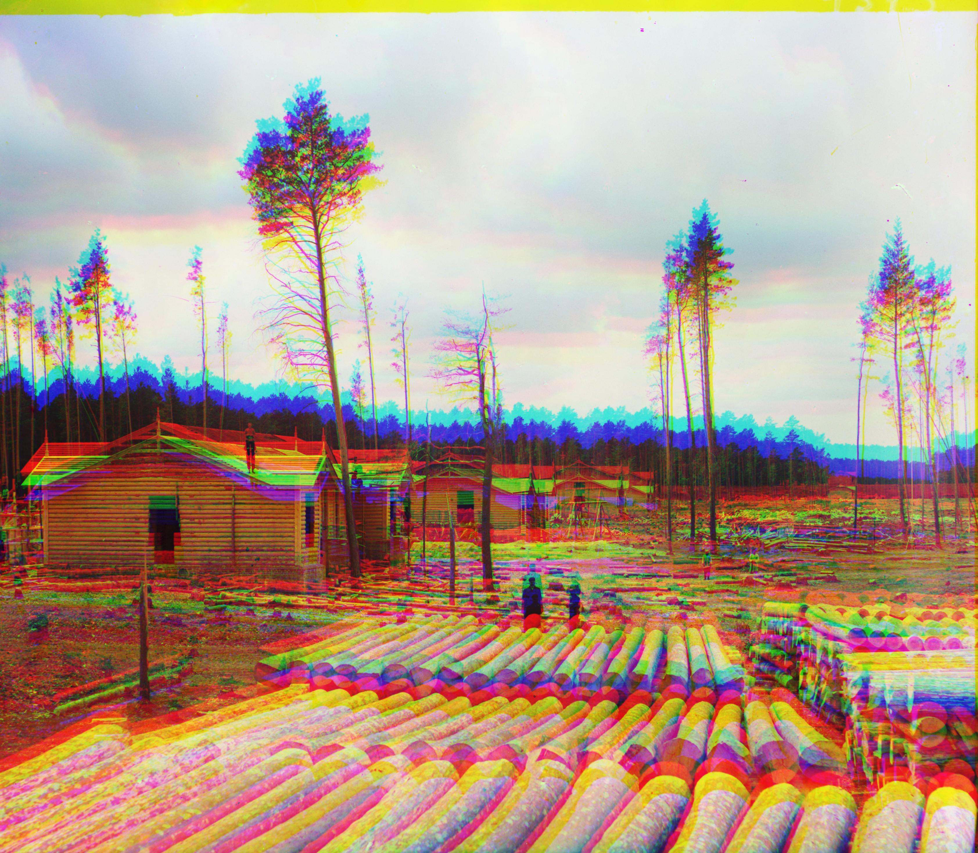
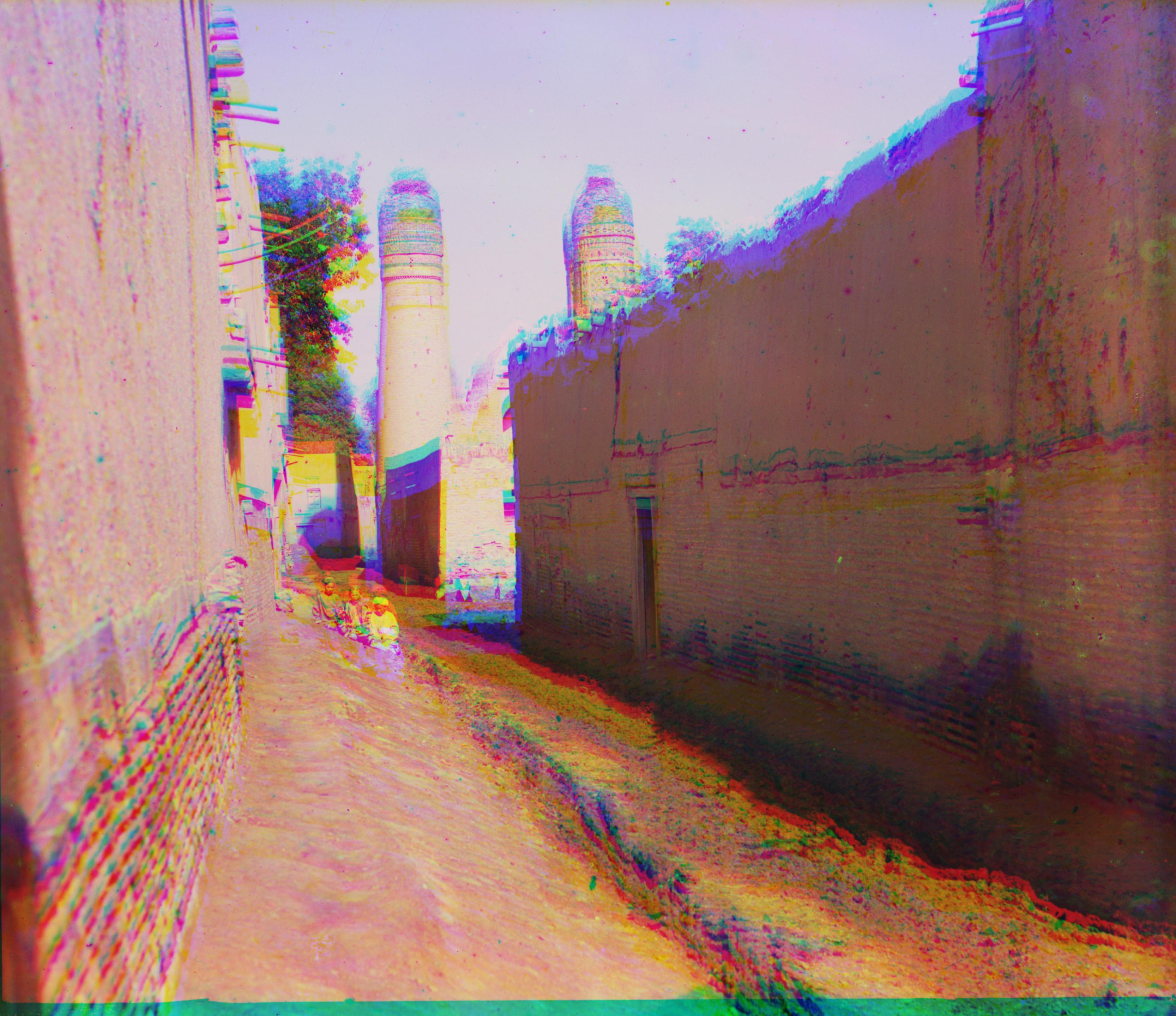
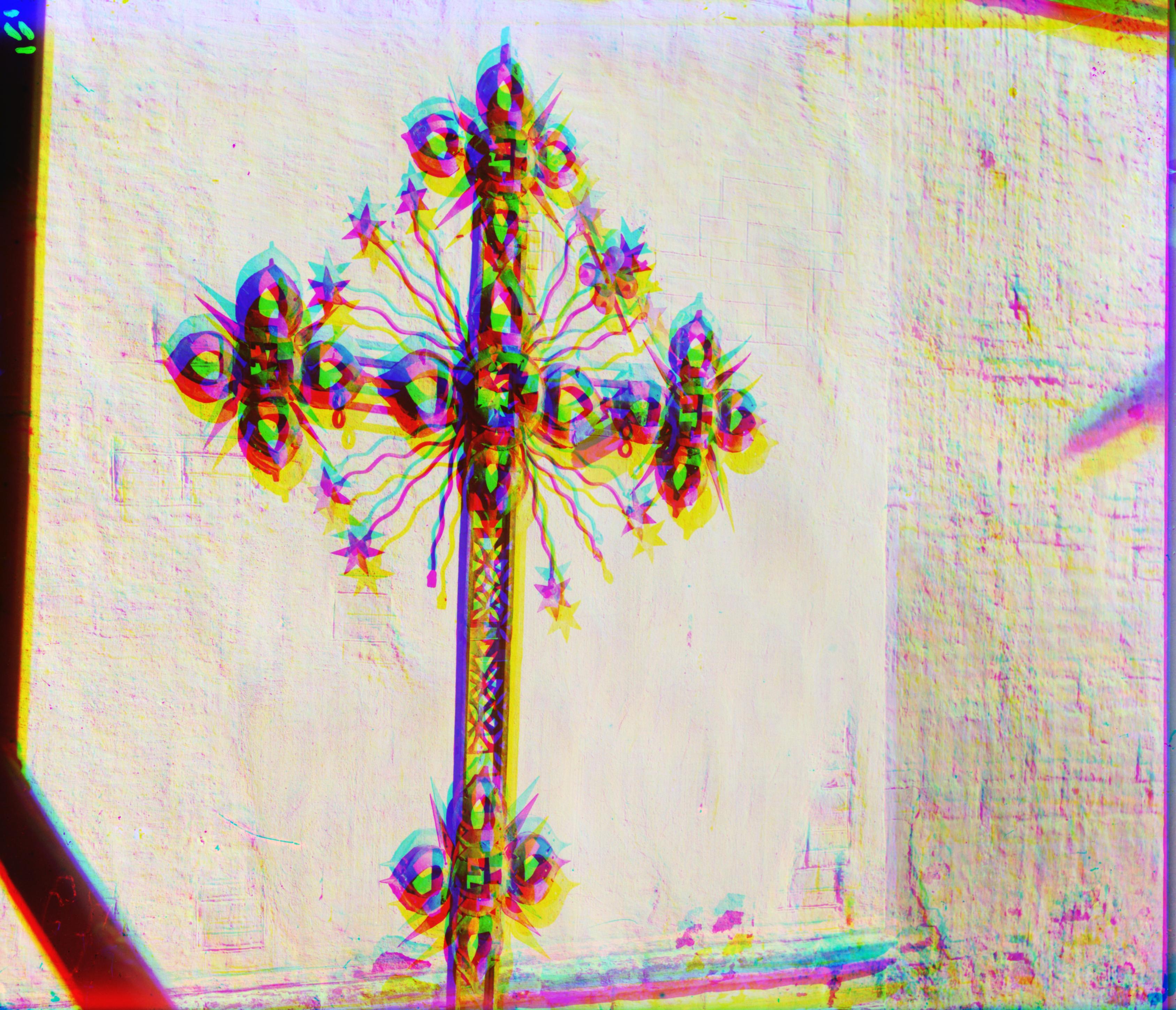
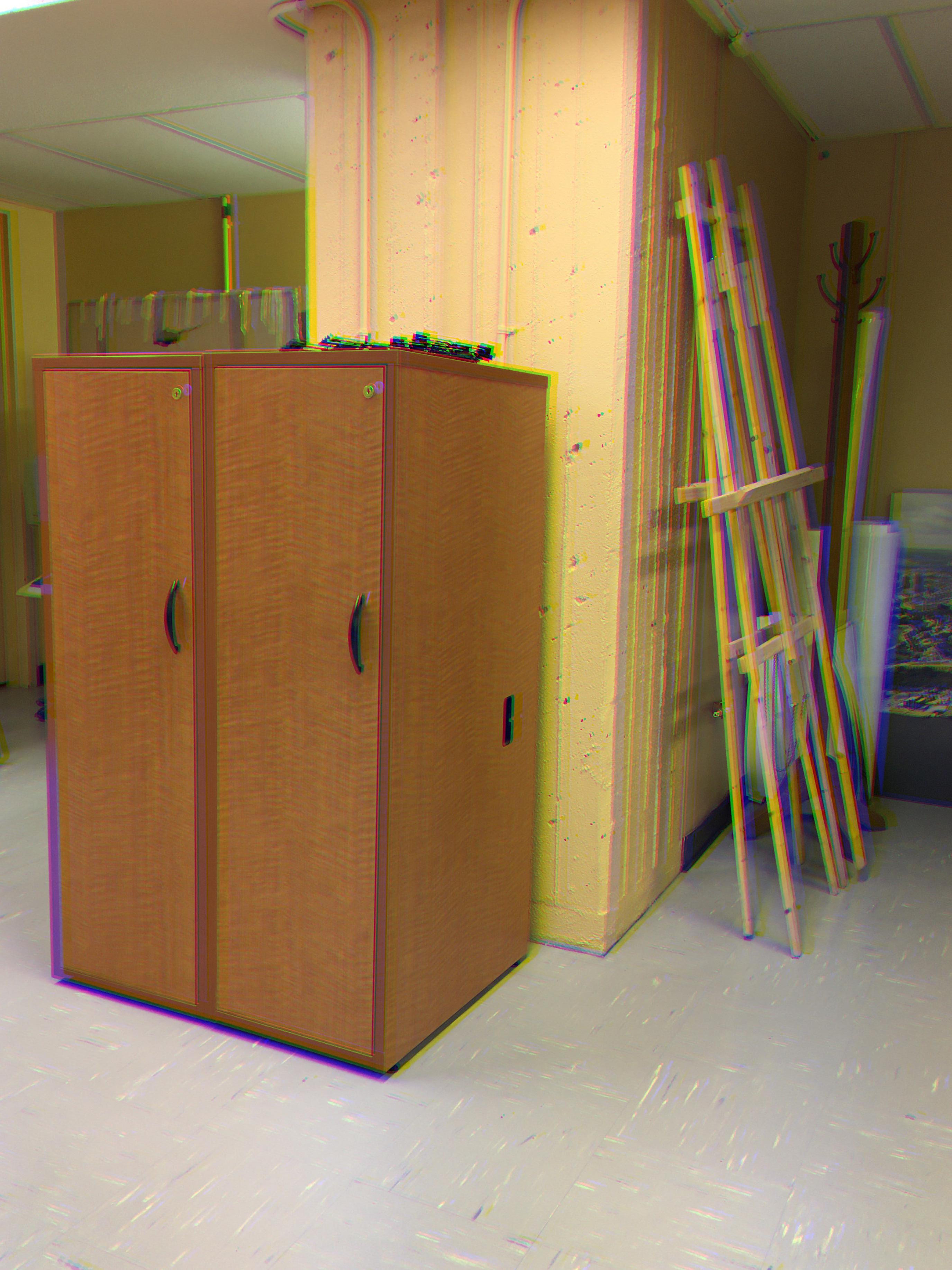
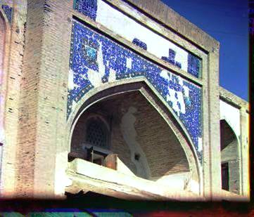
The results reveal the algorithm to work not perfectly. Manly, an incorrect shift of the blue channel is visible. Shift-estimation of the green channel was better in general. I can't really explain what lead to this incorrect estimate as the algorithm is the same as used for the first task. Moreover, shift detection on smaller scales works well in general, the misalignment only appears from scale 1:2 on upwards (i.e. on scale 1:2 and the original image). This is visible here:
| 
| 
| scale = 1:8 | scale = 1:4 | scale = 1:2 |
Maybe the kernel for the original image was still too small, although it is a 500 px x 500 px kernel.
One possibility is, that the correlation between blue and red is weaker than between red and green,
why the shift-estimation, that bases on this correlation, does not work perfectly.
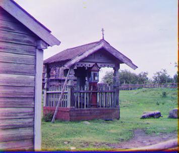
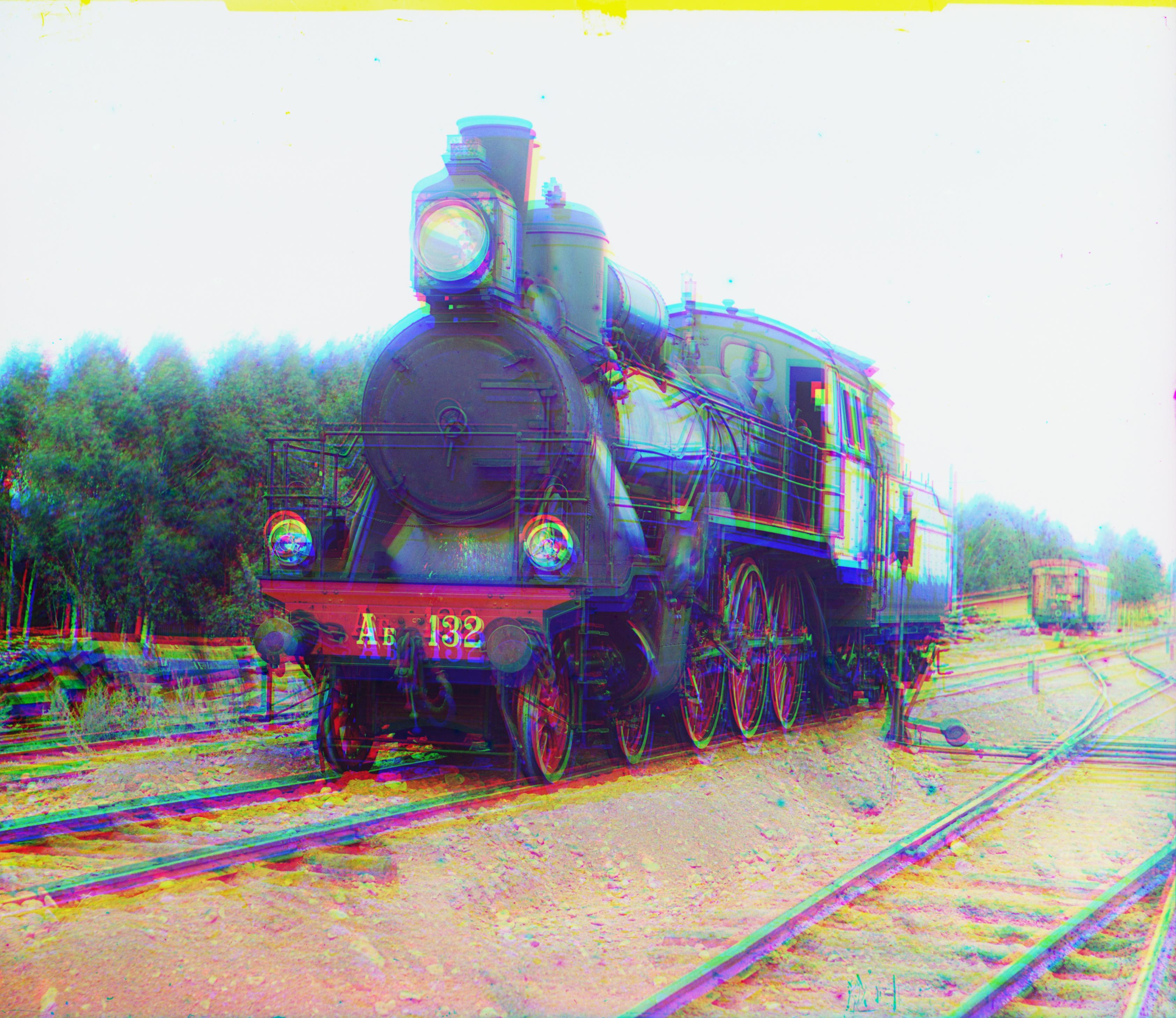
A general issue occurs if images show repetitive patterns (for example 00087u.tif) or large homogenous surfaces without distinct boarders in the area where the kernel is taken (00036u.tif, below). In the first case, shifting the kernel might lead to ambiguities.
Such issues can be met by setting the range for kernel-shifting to appropriate values. In case of large homogenous surfaces a larger kernel has to be chosen in order to cover boarders or more distinct structures.
Further images are:
| 
| 
| 
| 00008u.tif | 00036u.tif | 00068u.tif | 00075u.jpg |
| 
| 
| 
| 00835u.tif | 00970u.tif | 01228u.tif | 01235u.tif |
| 
| ||
| 01342u.tif | 01361u.tif |
| 
| 
|
|
|
|
|
|
| 
| 
| 
| 00106v.jpg | 00757v.jpg | 00888v.jpg | 00889v.jpg |
|
|
|
|
|
| 
| 
| 
| 000907v.jpg | 00911v.jpg | 01657v.jpg | 00889v.jpg |
|
| |||

| |||
| 01880v.jpg |
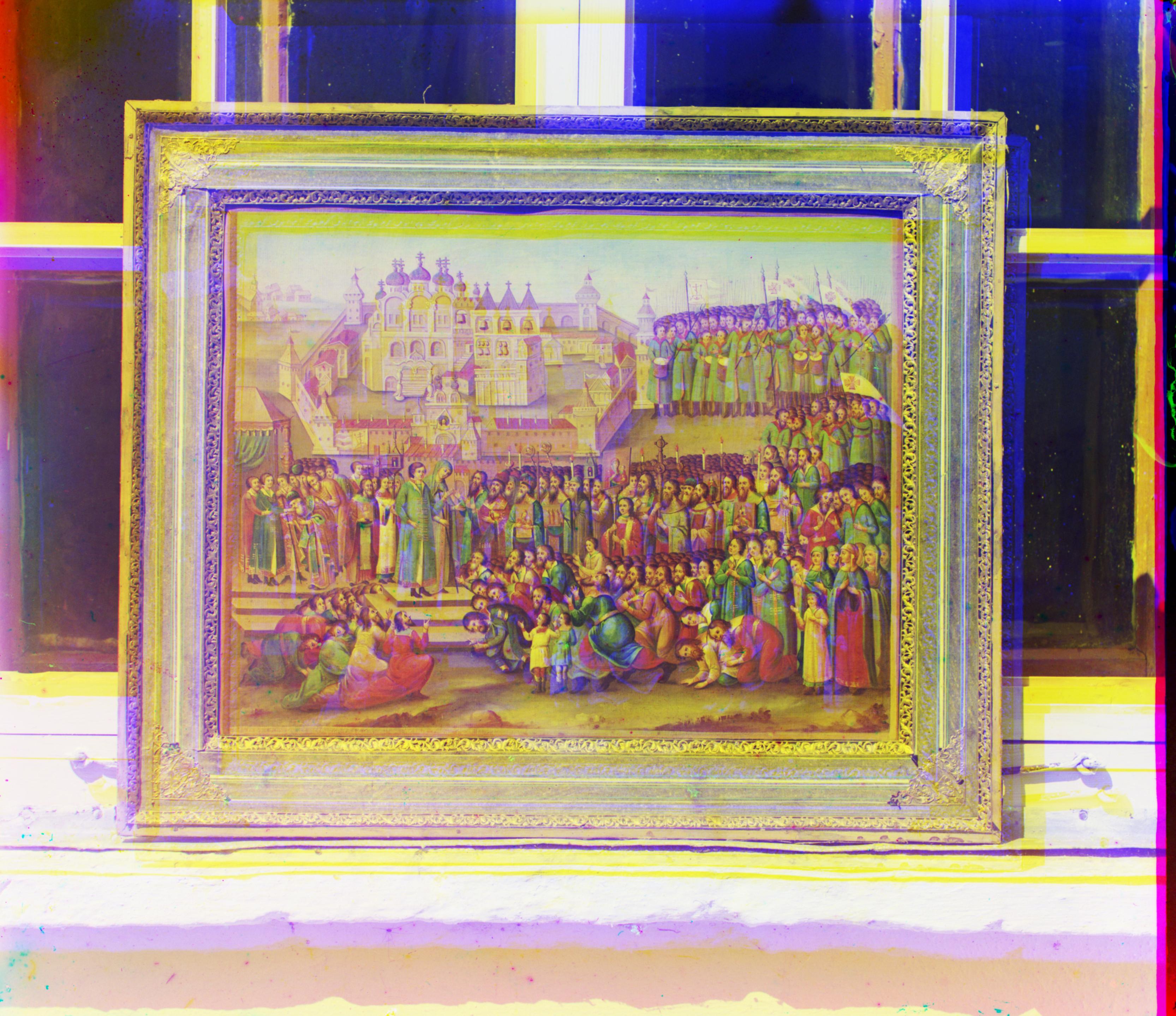
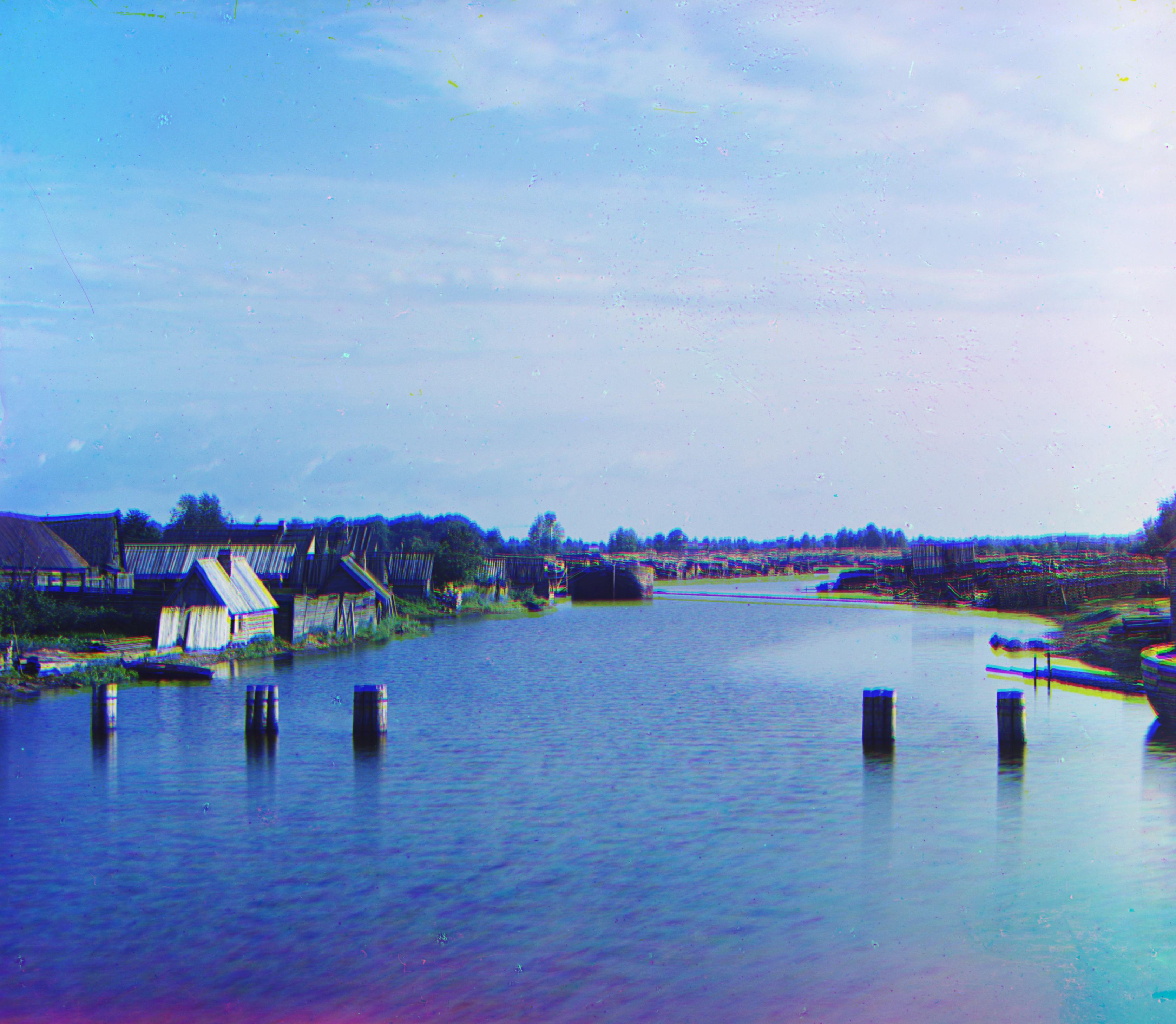
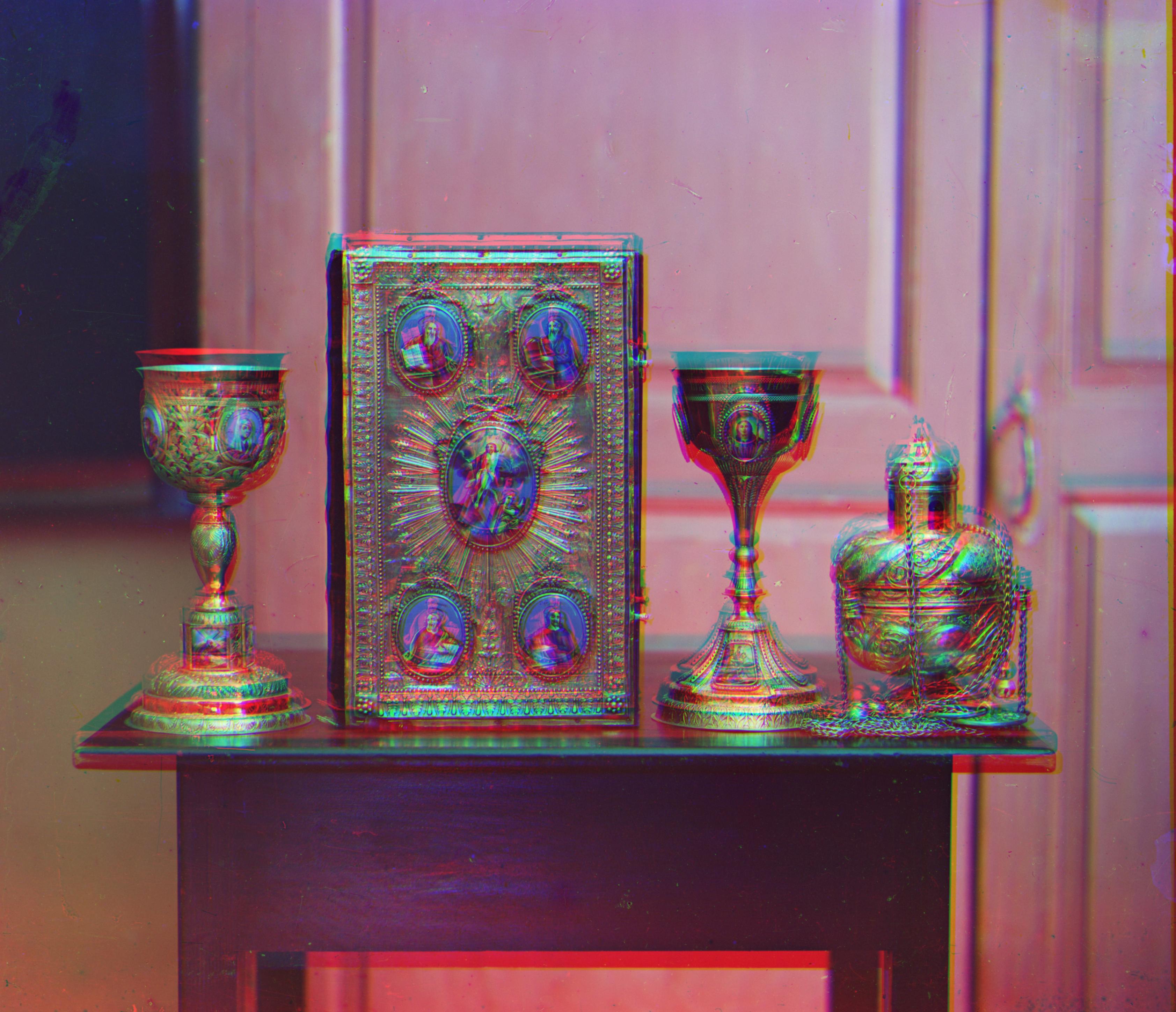
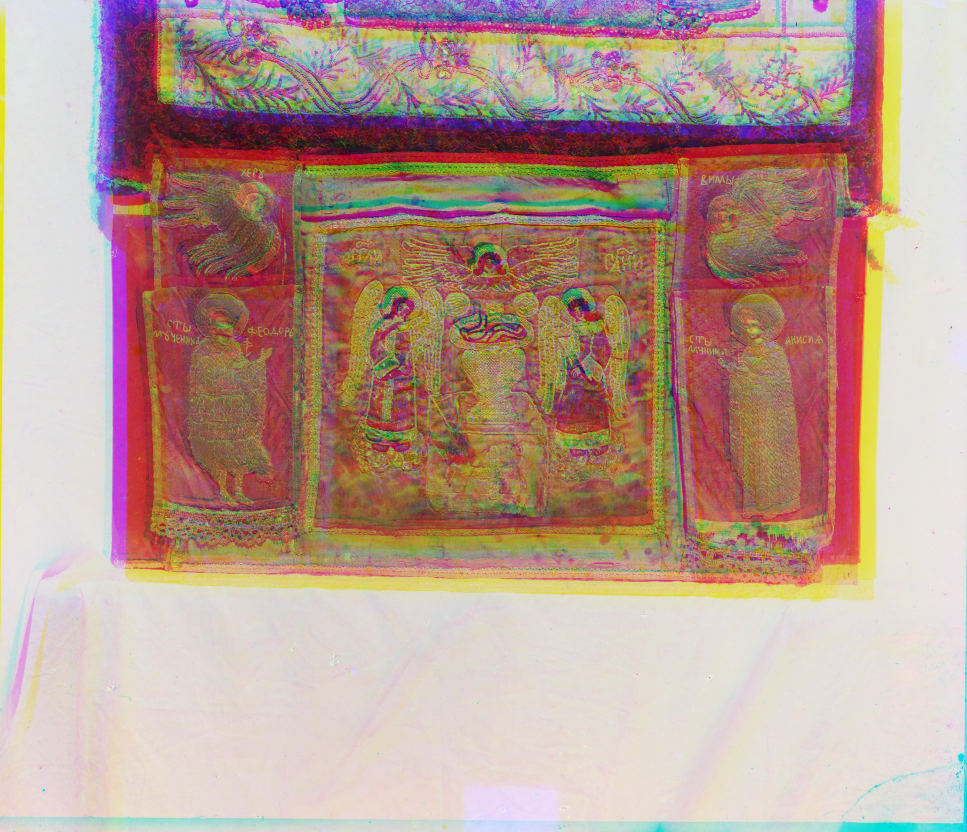
Second, I applied a white balance (WhiteBalance.m) correction, based on the gray-world assumption. I calculated the mean gray-value for every color and then brought the gray-value of the blue- and green-channel to the level of the red-channel. For some of the pictures, this correction results in images with too bright values (for example 01657v.jpg):
|
|
|
|
|
| 
| 
| 
| 00106v.jpg | 00757v.jpg | 00888v.jpg | 00889v.jpg |
|
|
|
|
|
| 
| 
| 
| 000907v.jpg | 00911v.jpg | 01657v.jpg | 00889v.jpg |
|
| |||
| |||
| 01880v.jpg |
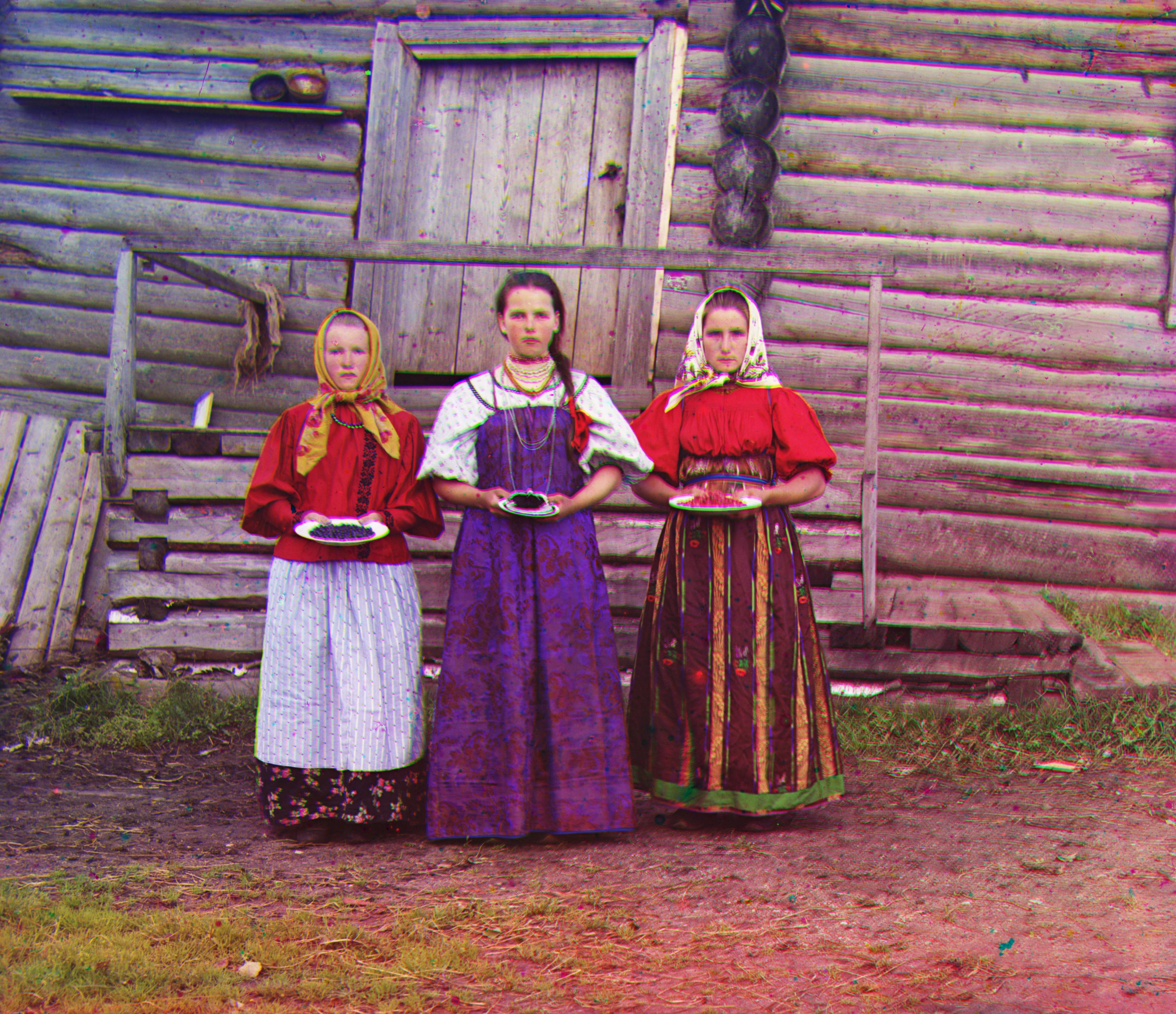
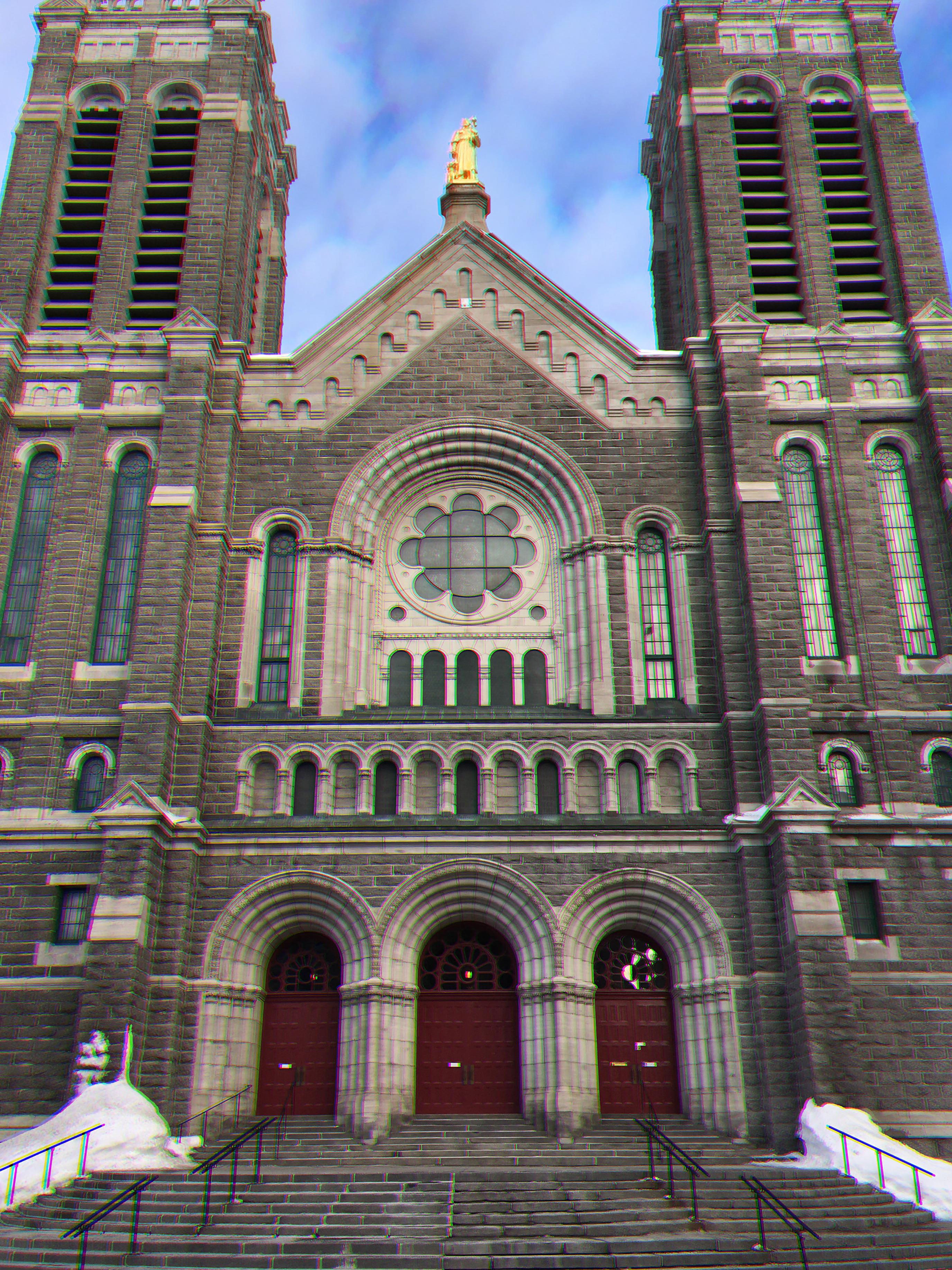
As a second auxiliary task, I detected and removed the frame of the images automatically (function: cut2boarders.m). Therefore, I used a Sobel-Filter in order to detect distinct gradients. From these gradients, I only selected the most distinct ones, because I assume the frames of the images to be distinct edges (Matlab-Function bwareaopen). This results in a first approximation of the boarders. As visible in the images below, the algorithm does not work well for all images, yet, but a better frame-detection is visible (top lines: originals, bottom: automatic edge-detection).
|
|
|
|
|

| 
| 
| 
| 00106v.jpg | 00757v.jpg | 00888v.jpg | 00889v.jpg |
|
|
|
|
|

| 
| 
| 
| 000907v.jpg | 00911v.jpg | 01657v.jpg | 00889v.jpg |
|
| |||

| |||
| 01880v.jpg |