The goal of this project is to reconstruct an RGB version of three monochromatic images taken separately from the same scene and (hopefully) the same position.
In order to do that one can try to find a (x,y) translation of two channels over a third one that minimizes a given metric. In this work I applied the Sum of Squared
Differences over two channels, and the results are shown below.
Results: Single Scale Approach
For the alignment of images of small size I performed a simple Sum of Squared Differences (SSD) between two channels where one is fixed and the other translated
vertically and horizontally in the interval [-15:15]. In order to obtain better results the border of the images are cropped before this comparison. The details of how
the crop is done is show in the "Additional Credits" Session.
00106v.jpg tG : x = 4 ; y = 1 tR : x = 9 ; y = 0
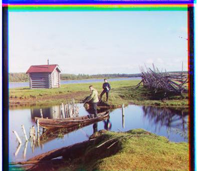
00757v.jpg tG : x = 2 ; y = 3 tR : x = 5 ; y = 5
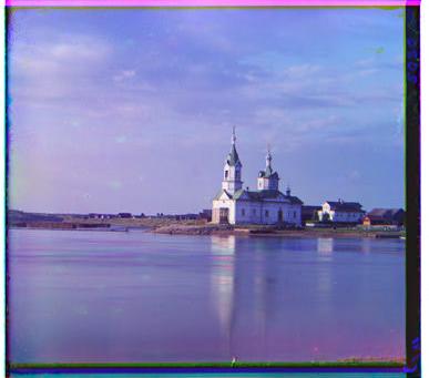
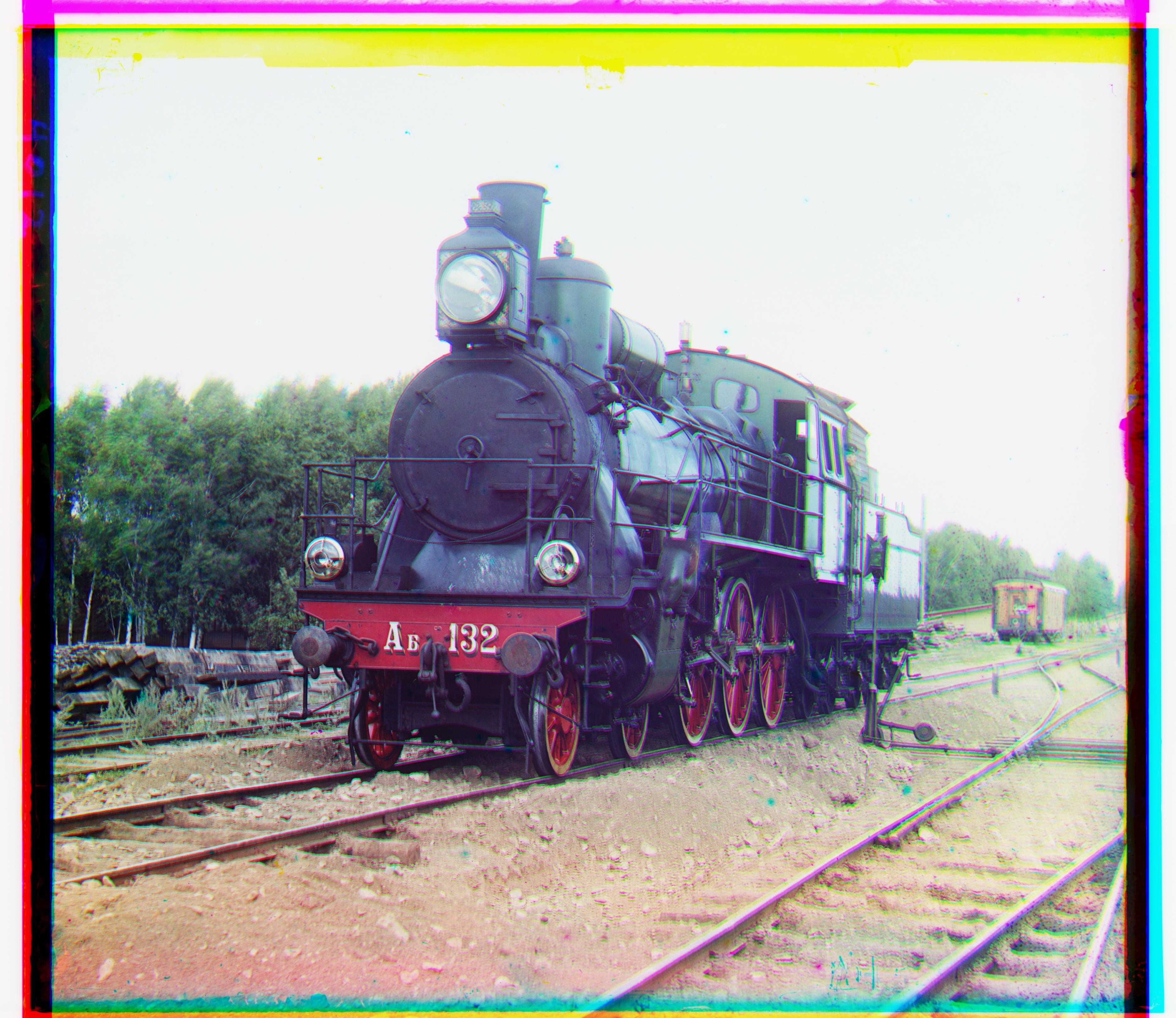
00888v.jpg tG : x = 6 ; y = 1 tR : x = 12 ; y = 0
00889v.jpg tG : x = 2 ; y = 2 tR : x = 4 ; y = 3
00907v.jpg tG : x = 2 ; y = 0 tR : x = 5 ; y = -1
00911v.jpg tG : x = 1 ; y = -1 tR : x = 13 ; y = -1
01031v.jpg tG : x = 1 ; y = 1 tR : x = 4 ; y = 2
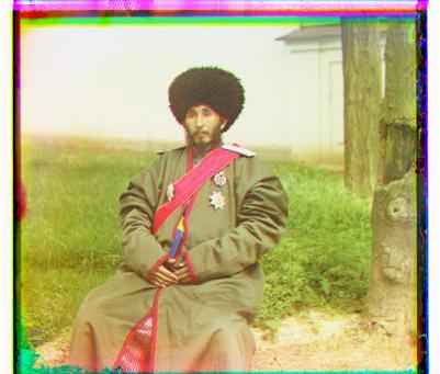
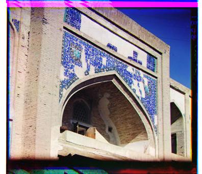
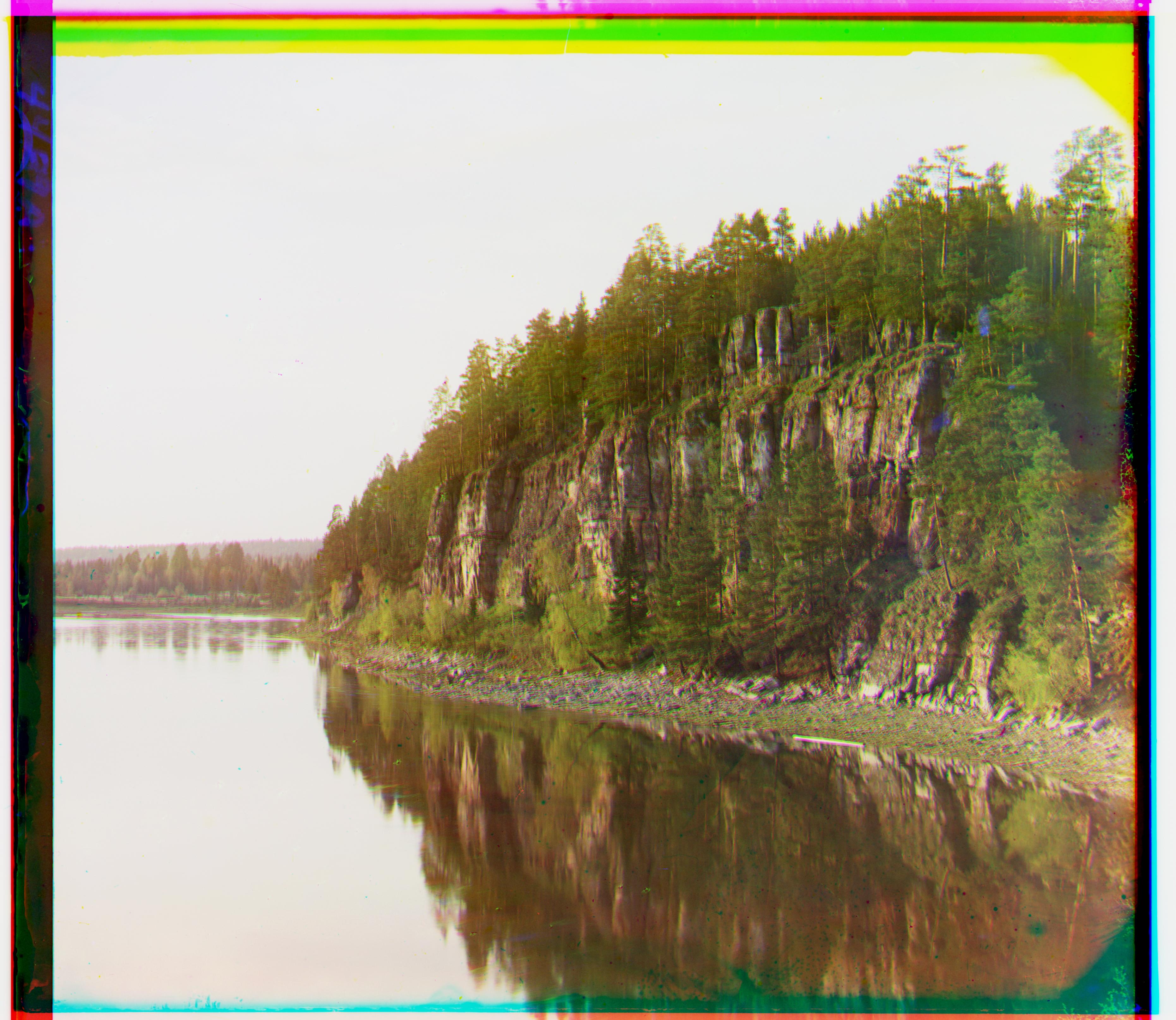
01657v.jpg tG : x = 6 ; y = 0 tR : x = 11 ; y = 0
01880v.jpg tG : x = 6 ; y = 2 tR : x = 14 ; y = 4
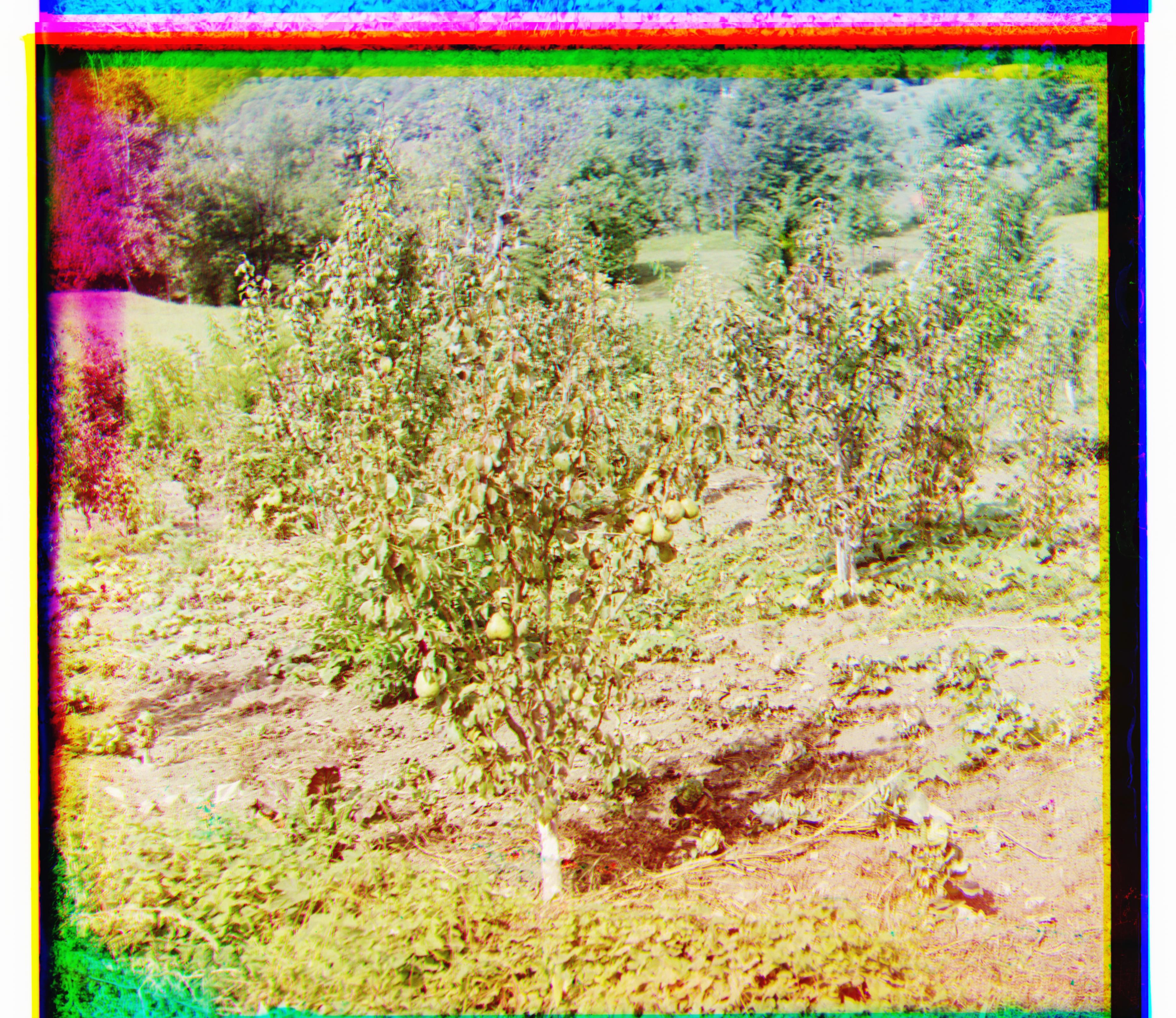
Results: Multiple Scales Approach
In order to deal with the larger size of the pictures I implemented the suggested idea of a pyramid of images. In this case the image is reduced to 10%, 20% and 30% of
its original size. To compare the cost of translating images with different sizes I scaled the SSD by the square of the scale factor. The translation that presents the
smallest cost is then scaled back to the original image size in order to have the desired translation effect.
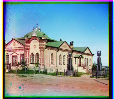
00029u.jpg tG : x = 40 ; y = 20 tR : x = 90 ; y = 40
00087u.jpg tG : x = 50 ; y = 40 tR : x = 110 ; y = 60
00128u.jpg tG : x = 30 ; y = 20 tR : x = 50 ; y = 40
00458u.jpg tG : x = 40 ; y = 0 tR : x = 90 ; y = 30
00737u.jpg tG : x = 10 ; y = 0 tR : x = 50 ; y = 10
00822u.jpg tG : x = 60 ; y = 20 tR : x = 130 ; y = 30
00892u.jpg tG : x = 20 ; y = 0 tR : x = 40 ; y = 0
01043u.jpg tG : x = -20 ; y = 10 tR : x = 10 ; y = 20
01047u.jpg tG : x = 20 ; y = 20 tR : x = 70 ; y = 30
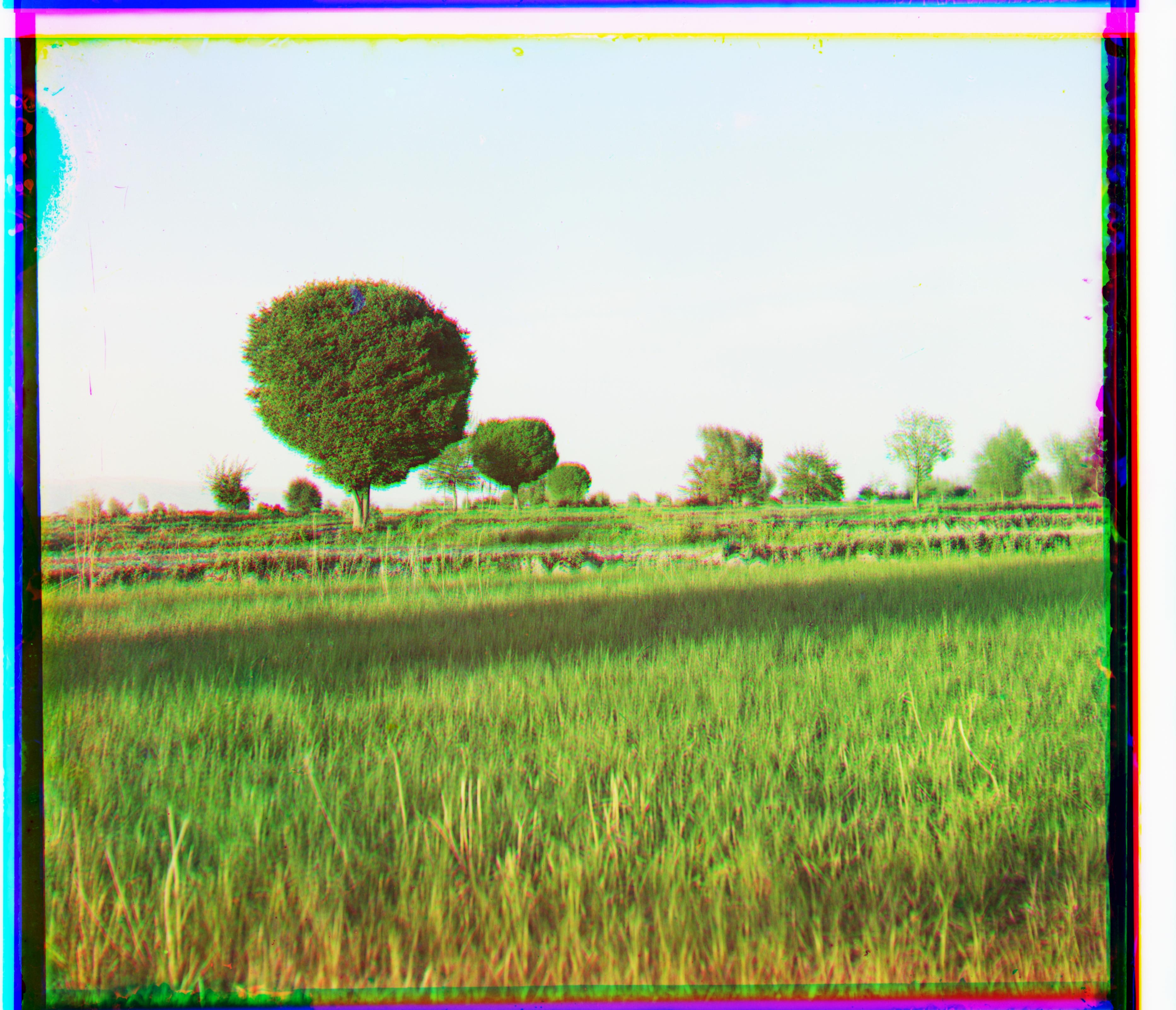
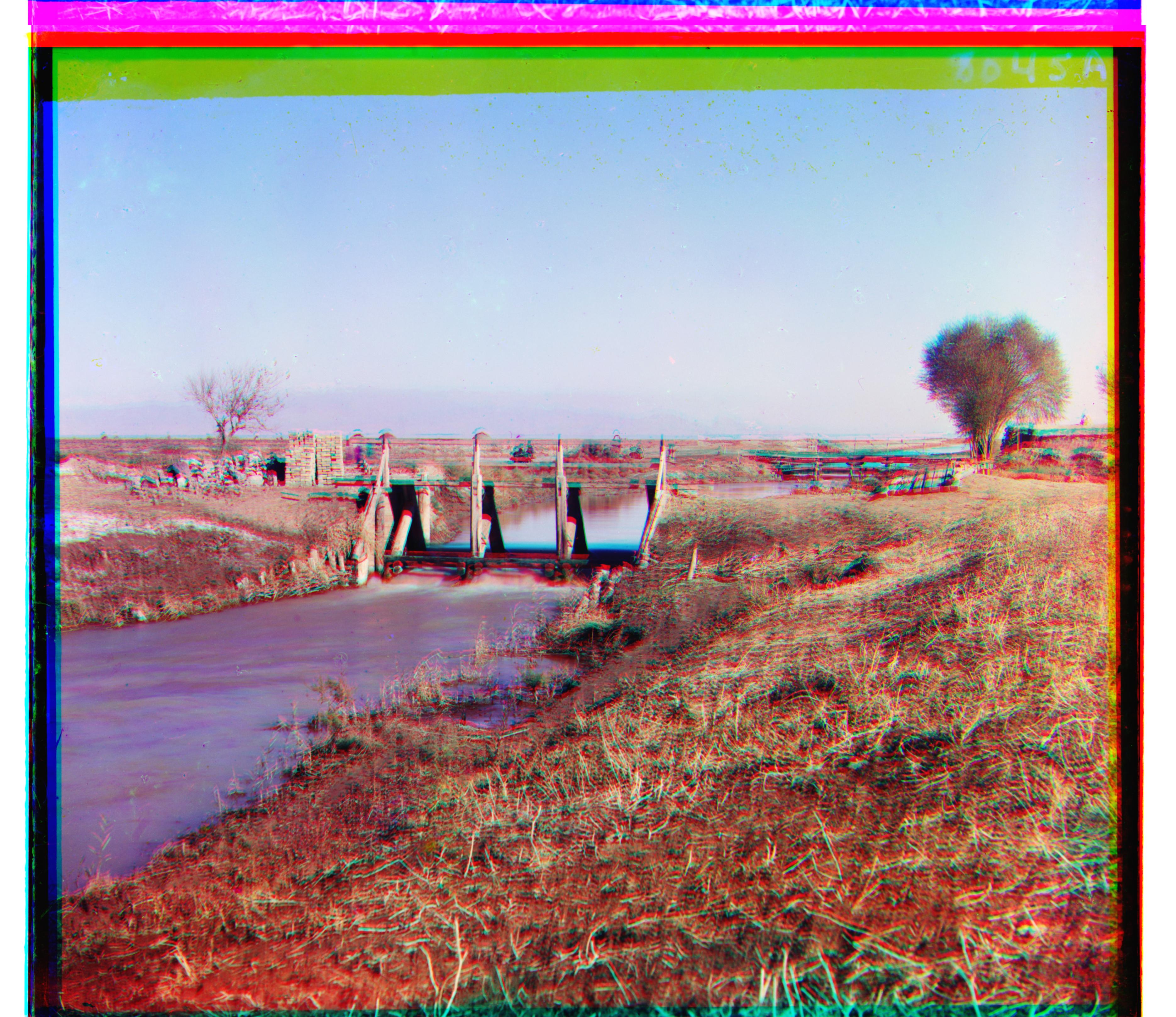
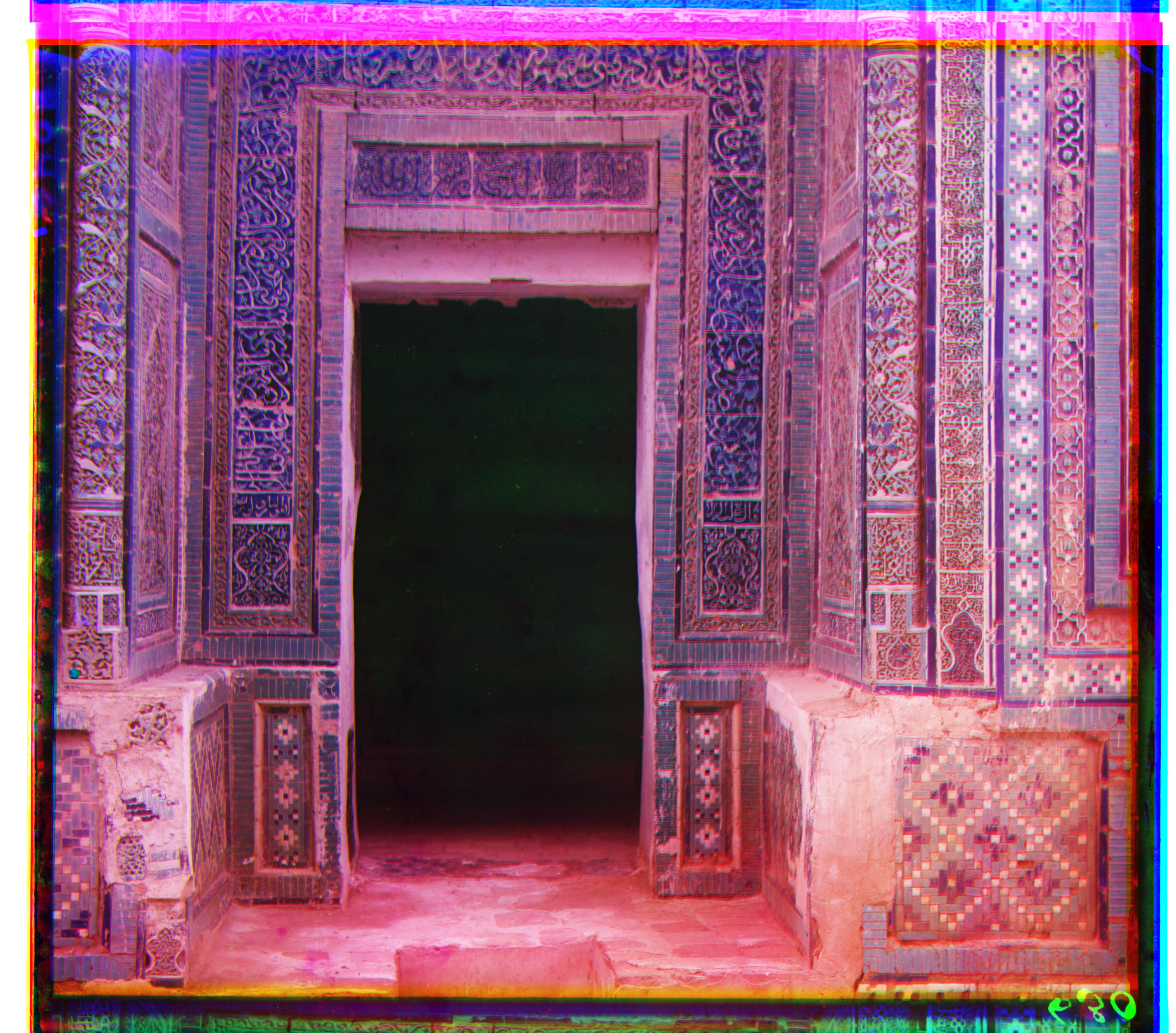
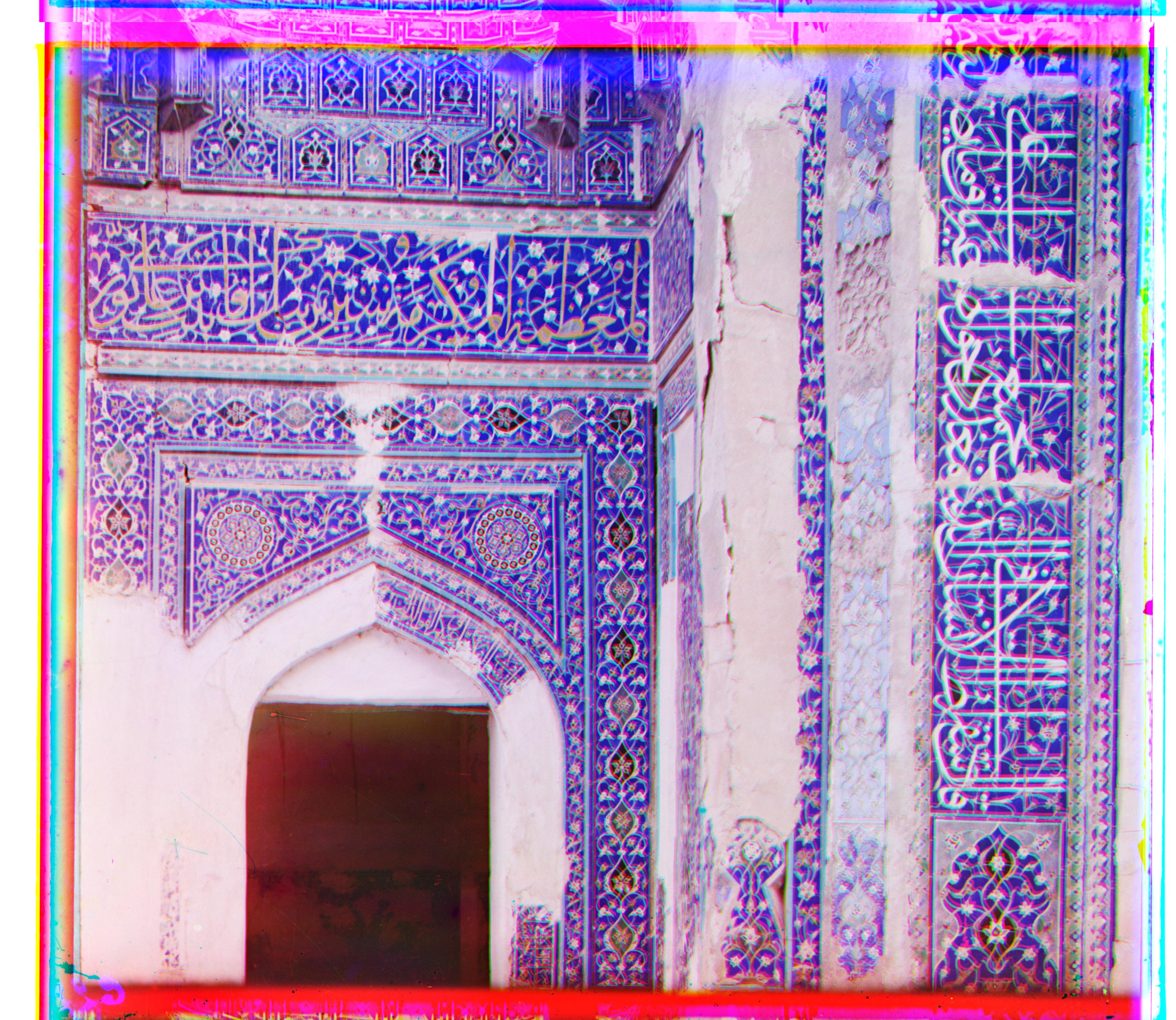
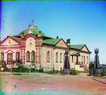
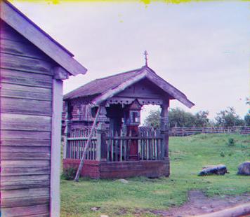
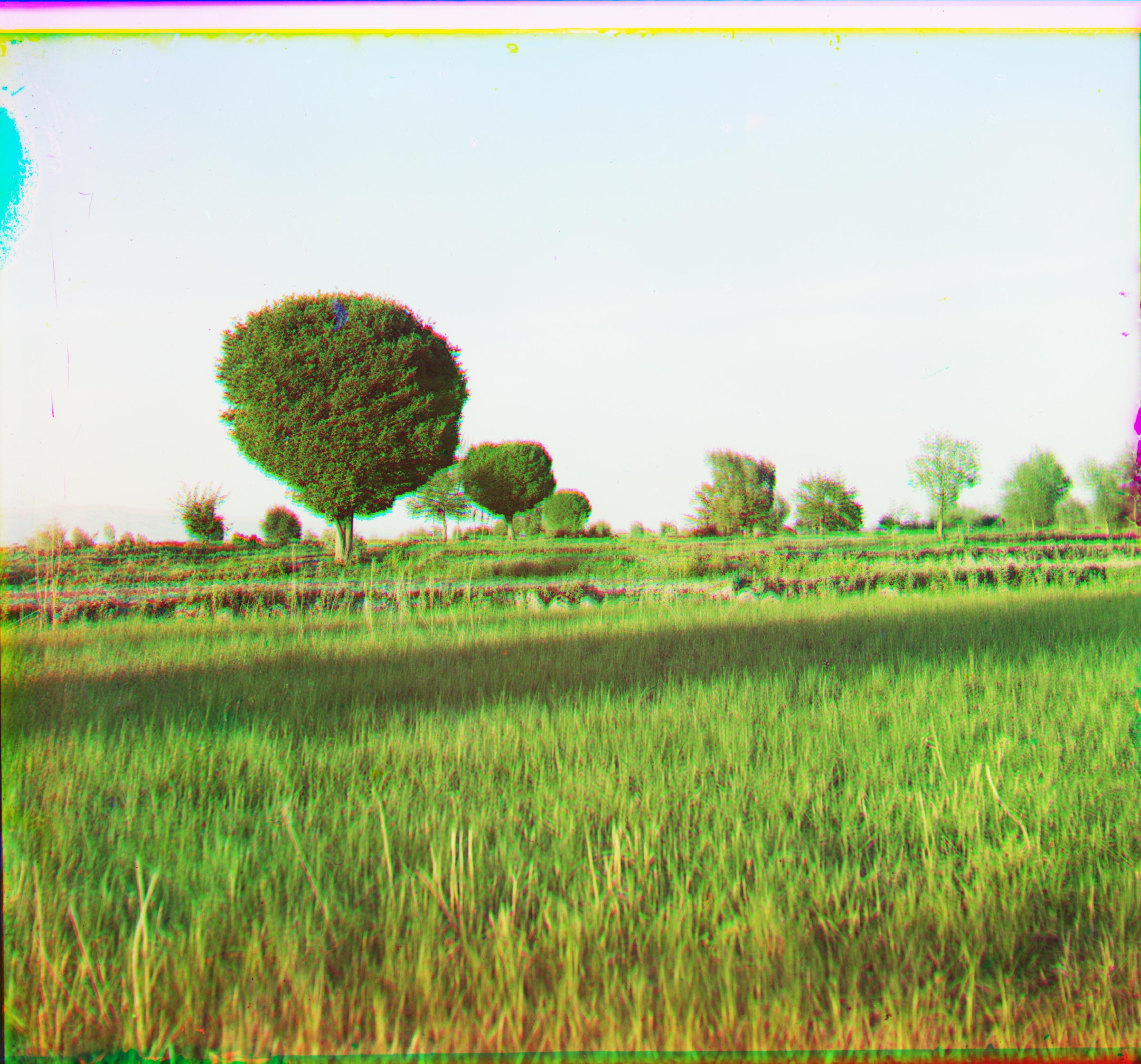
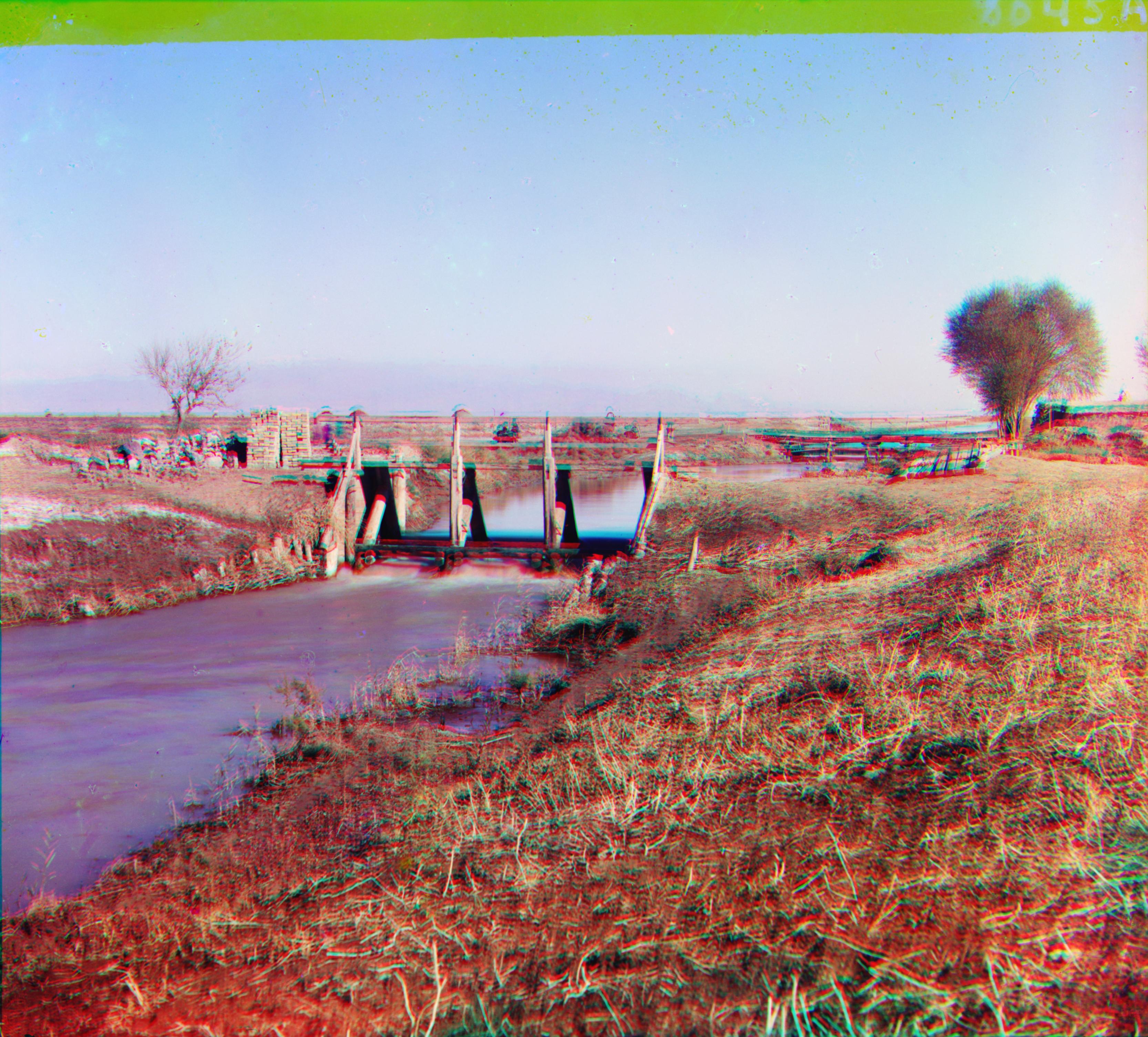
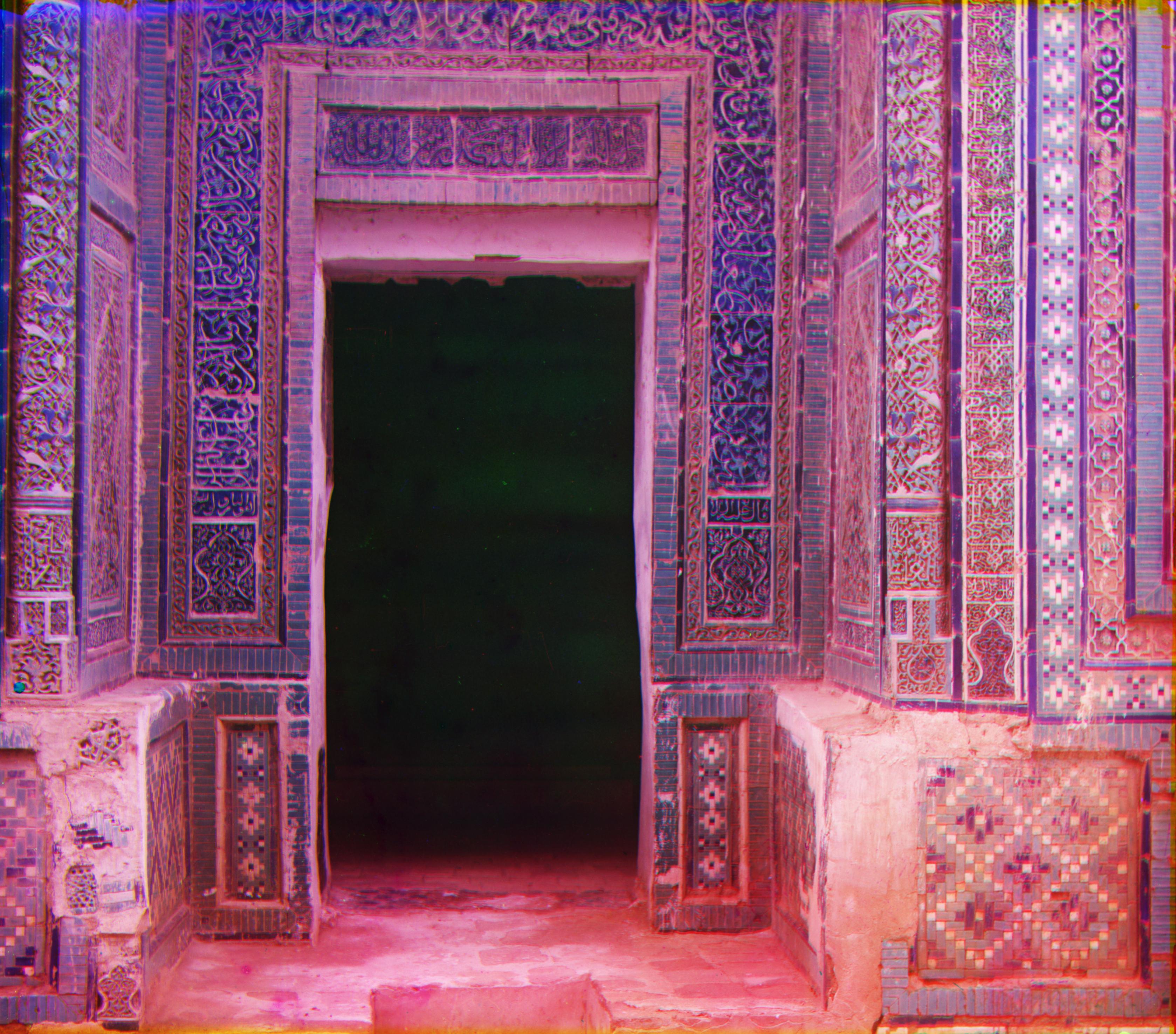
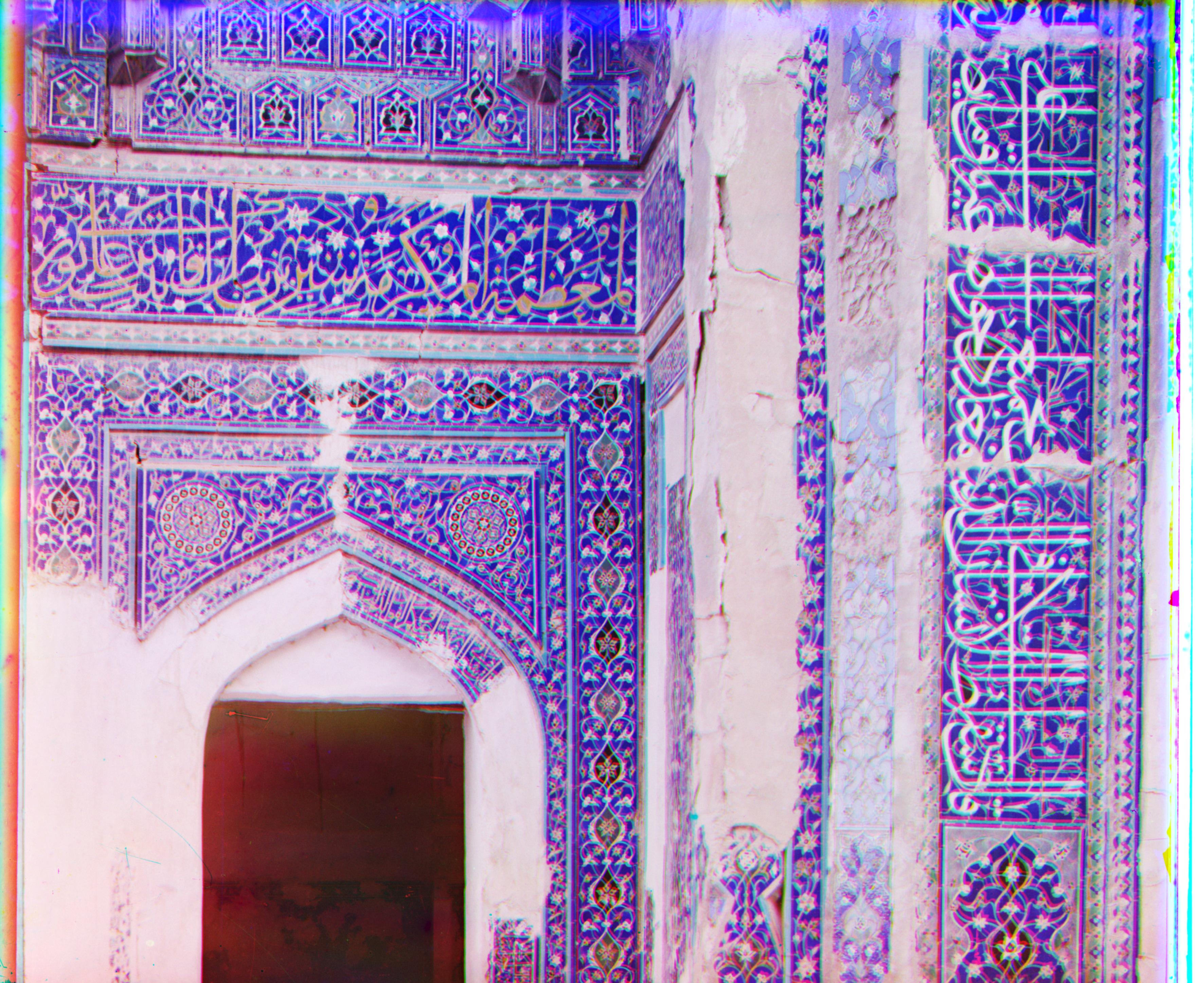
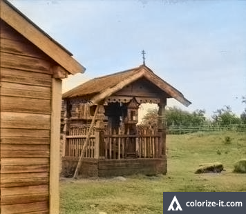
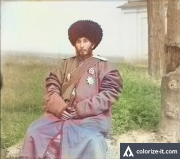
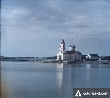
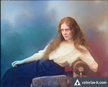
Results: Multiple Scales Approach (10 extra images from lcweb2.loc.gov)
Here are the results on more images from the provided dataset.
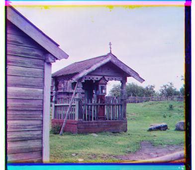
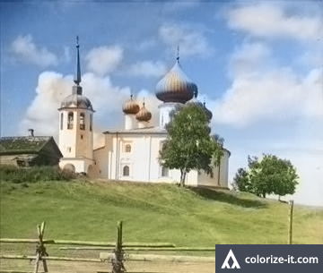
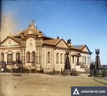
01670u.jpg tG : x = 60 ; y = 0 tR : x = 120 ; y = 0
01687u.jpg tG : x = 30 ; y = -10 tR : x = 140 ; y = -30
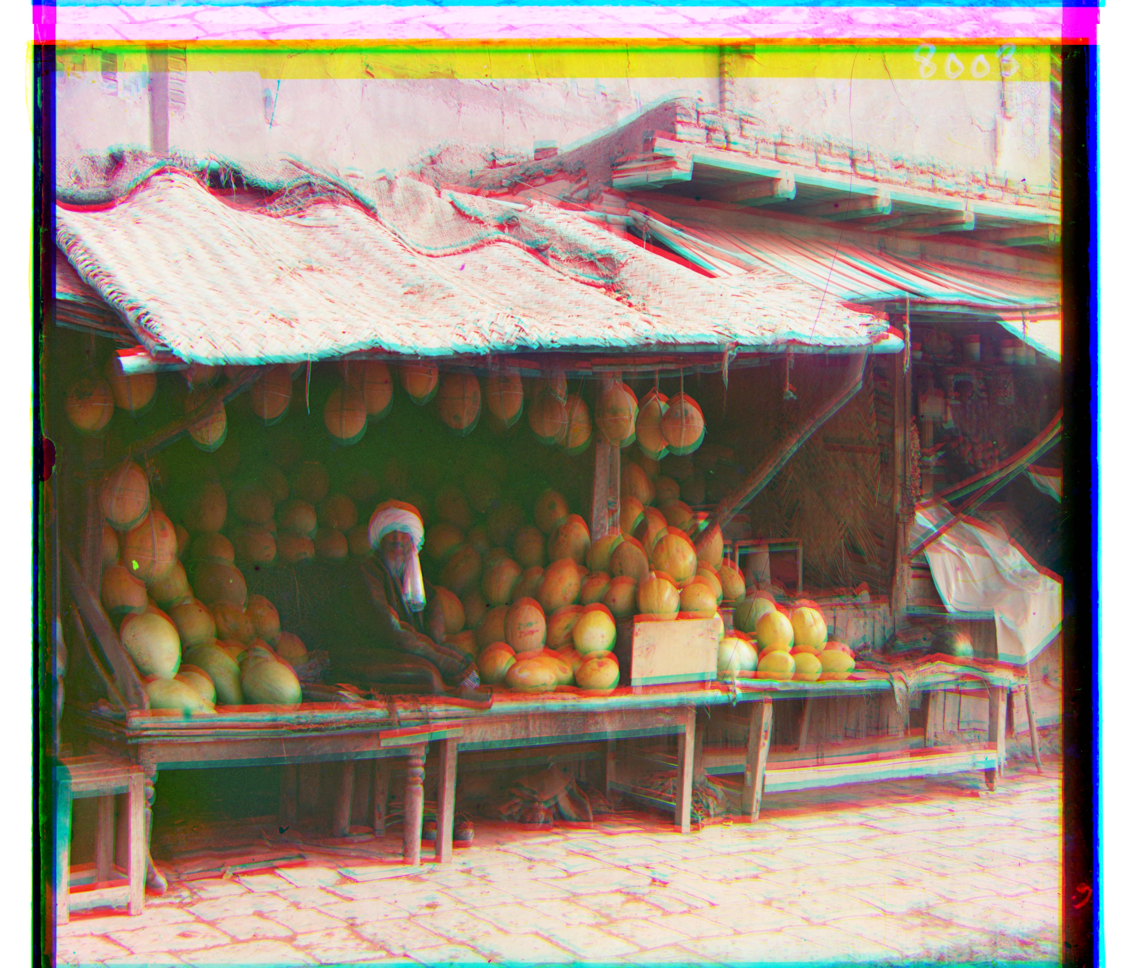
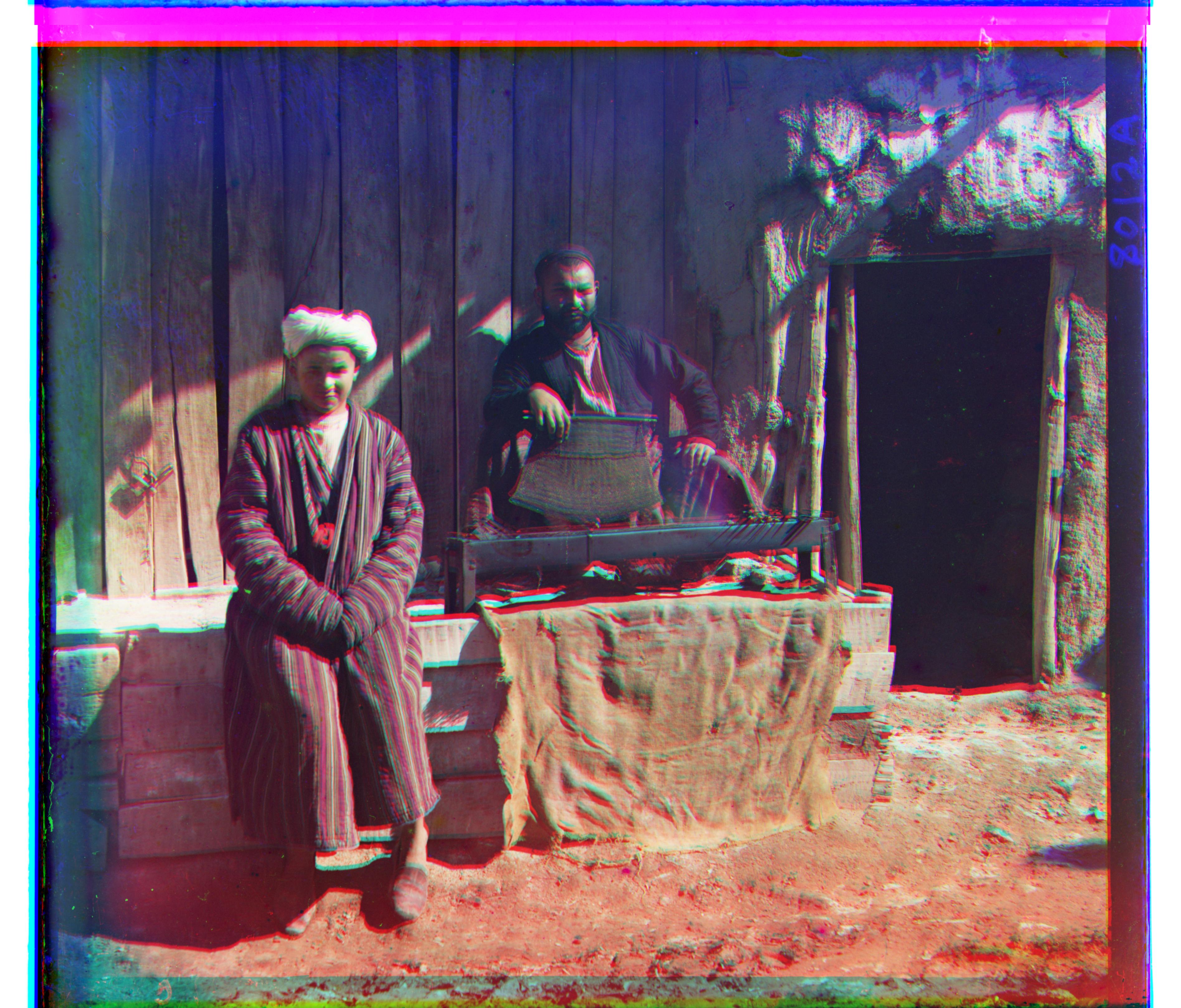
01707u.jpg tG : x = 70 ; y = 10 tR : x = 140 ; y = 0
01728u.jpg tG : x = 80 ; y = 10 tR : x = 150 ; y = 10
01748u.jpg tG : x = 80 ; y = 0 tR : x = 150 ; y = -10
01772u.jpg tG : x = 0 ; y = 20 tR : x = 0 ; y = 30
01791u.jpg tG : x = 40 ; y = -20 tR : x = 120 ; y = -50
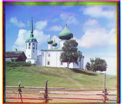
01814u.jpg tG : x = 80 ; y = 10 tR : x = 150 ; y = 10
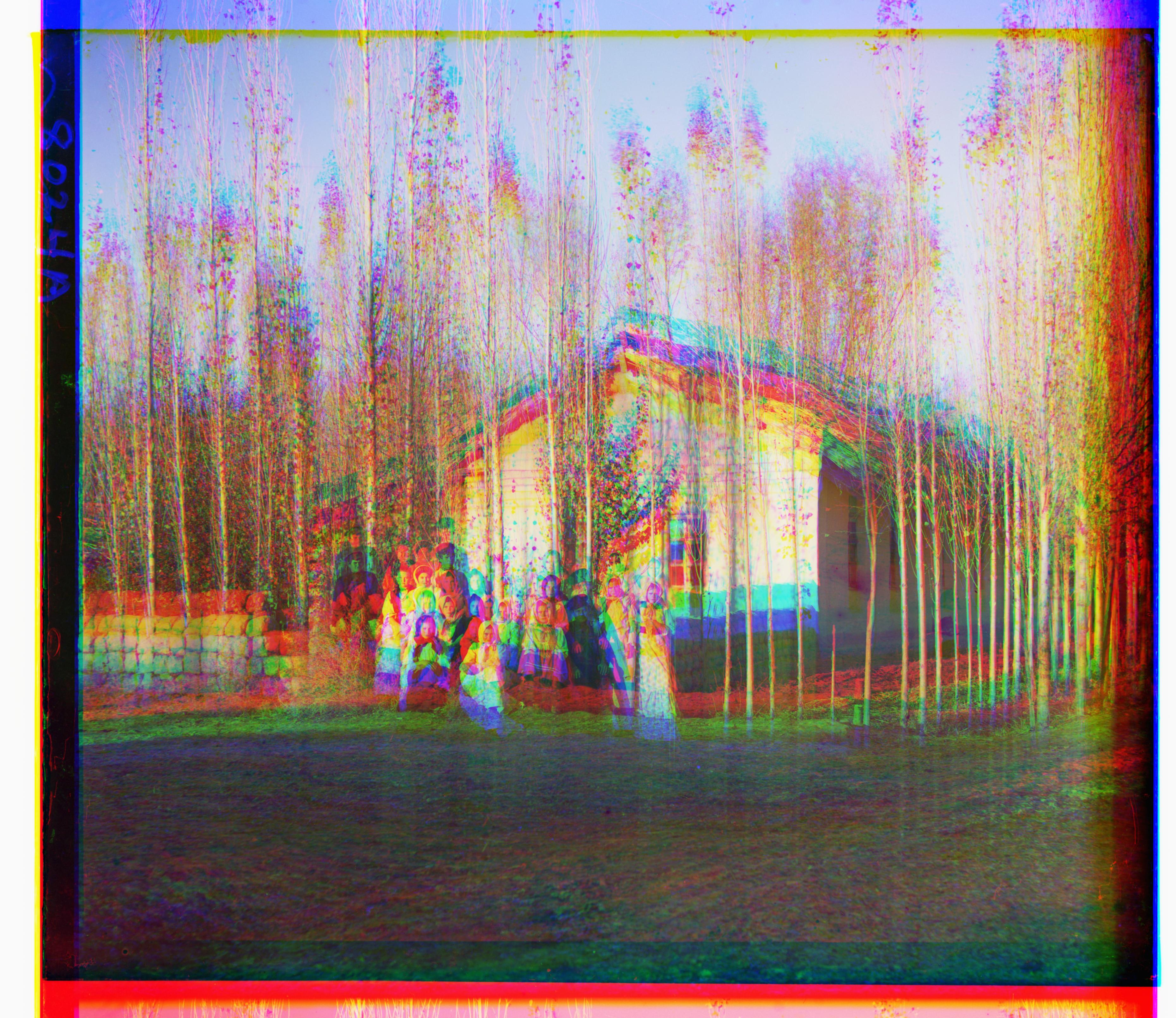
01815u.jpg tG : x = 70 ; y = 30 tR : x = 140 ; y = 60
01816u.jpg tG : x = 70 ; y = 30 tR : x = 150 ; y = 80
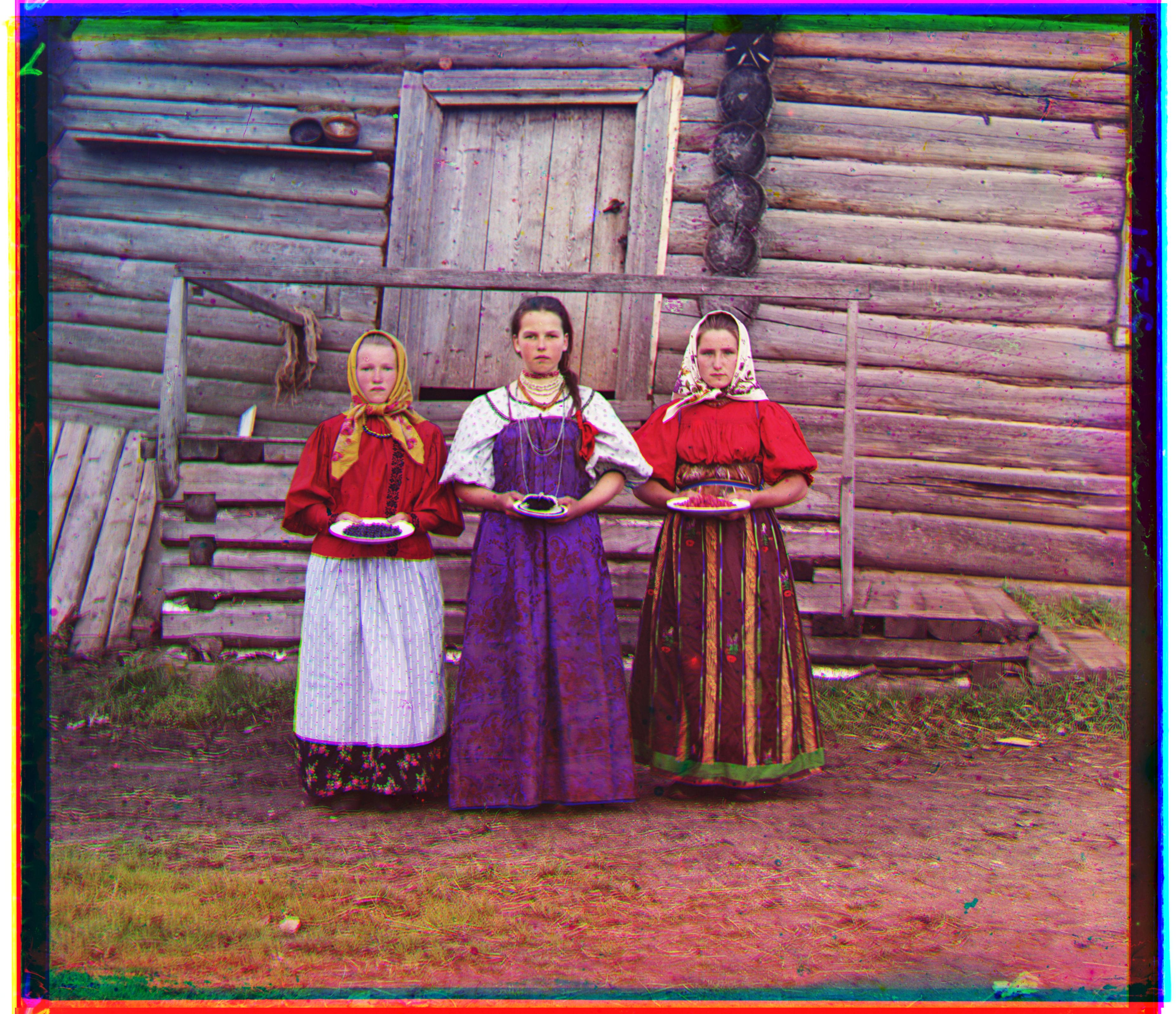
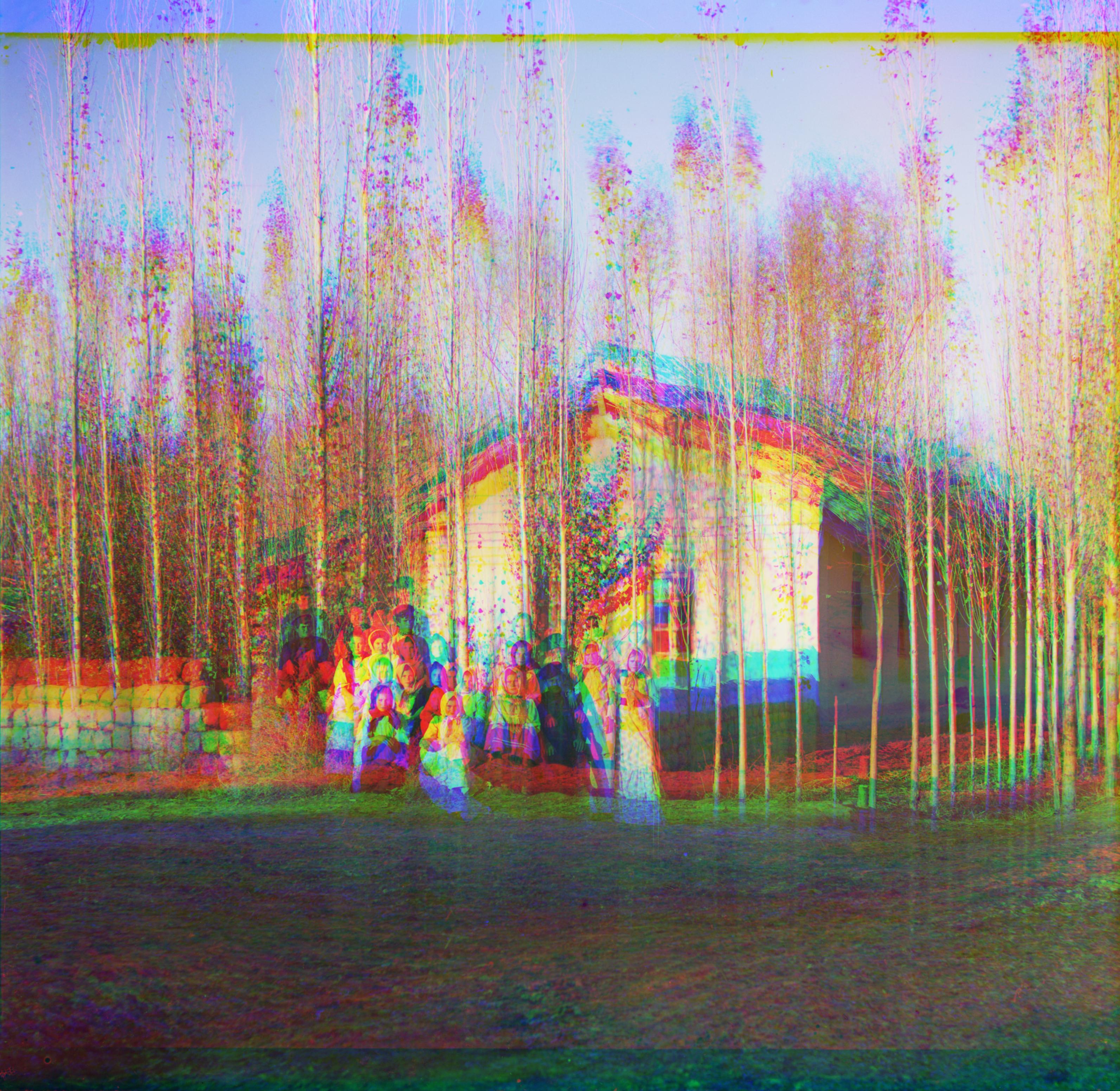
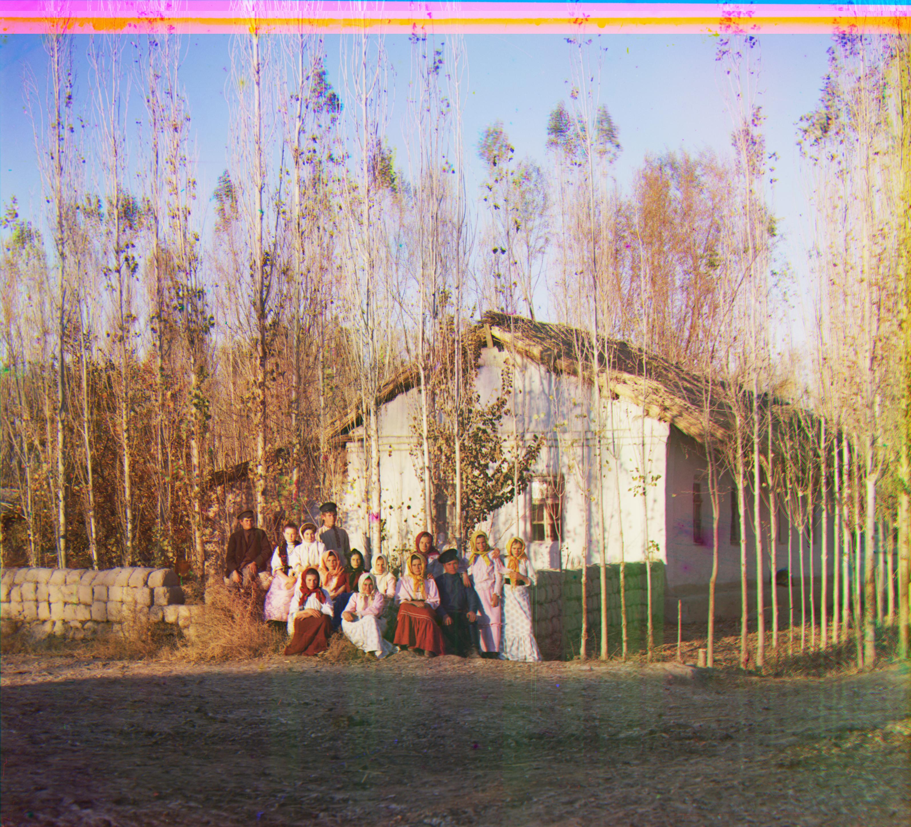
Results: Put yourself in the shoes of Prokudin-Gorskii!
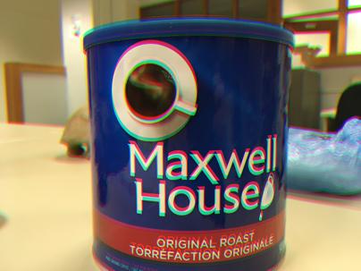
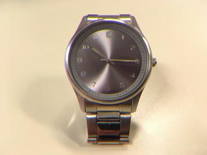
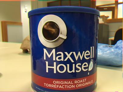
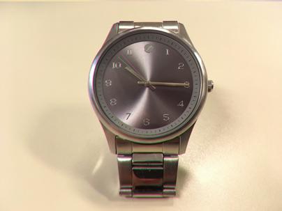
Here are the results of applying the technique on images I took myself.
original 0.jpg
original 1.jpg
original 2.jpg
0.jpg tG : x = 0 ; y = 1 tR : x = 1 ; y = 2
1.jpg tG : x = -1 ; y = -1 tR : x = 3 ; y = -2
2.jpg tG : x = 2 ; y = 0 tR : x = 2 ; y = 0
Additional Credits(1): Cropping borders
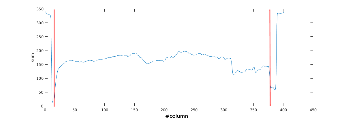
In order to the rid of the borders I implemented a discontinuity detector in the vertical and horizontal directions. For every image channel I perform the sum
of intensities of all columns. Next I check which of the columns in the first 10% and the last 90% of the image columns pass the following test:
where "column_i" is the column index and "all_columns" is the vector containing the sum of every column. I take the rightmost and leftmost value of the columns
that passed this test and decide the image will be cropped at those locations. In the following image it is possible to see the blue column indicating the sum for
every column in the x axis. The red lines indicate where the image was cropped.
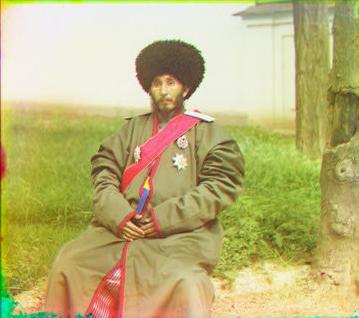
Original image.
Detected vertical borders on the red line location.
The following pictures are the result of applying the automatic crop algorithm.
00106v.jpg
00757v.jpg
00888v.jpg
01791u.jpg
01814u.jpg
01815u.jpg
Additional Credits(2): Channels alignment by measuring the image sharpness
One can measure the image sharpness by taking the average of the gradient magnitude. The idea was then measure the sharpness of an image composed by two channels overimposed.
Ideally two perfectly aligned channels would present a high sharpness since the edges will be more well defined than with two channels badly aligned. The results show that this
metric can estimate better alignment for most of the images.
01772u.jpg aligned with SSD.
01772u.jpg aligned with the sharpness metric.
01816u.jpg aligned with SSD.
01816u.jpg aligned with the sharpness metric.
00458u.jpg aligned with both methods. It is possible to see that the alignment with SSD gives better results at the train while the alignment with the sharpness measurement gives better results at the bottom left train track.
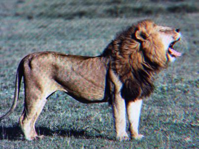
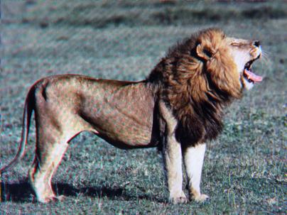
Additional Credits(3): Colorization with deep learning
Here I used a deep neural network to estimate colors from a greyscale version of the rgb output of the algorithm. The results can be seen bellow.
Source: Colorize-photos