HW6: Stereo Light Probe
GIF-4105/7105 H2017
Author: Henrique Weber
One of the main goals of Computer Graphics is to virtually recreate the real world. One way to do this is to use pictures (more specifically equirectangular pictures) as light sources by projecting the pixels intensities on the virtual objects. These special pictures, also called in this context environment maps, can create very realistic results, and can be approximated by only a single picture (ideally with high dynamic range) of a spherical mirror.
However one of the main drawbacks of this approach is that the lighting effects remain coherent only when the object is rendered exactly where the spherical mirror ball was in the original scene. If this is not the case the lighting effects become incoherent regarding the environment that was used as light source. To overcome this problem in a simple way, Corsini et al. proposed in the paper intitulated Stereo Light Probe to use two calibrated spherical mirrors to locate the position of light sources in space. In this project, I implemented a similar version of the proposed method and discuss its pros and cons.
Part 1: Acquisition method
To acquire the data for this project I rendered synthetic scenes with known location of both mirror balls and light sources. Such approach allowed a better understanding of the problem and also a more accurate comparison between the results and the ground truth.
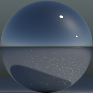
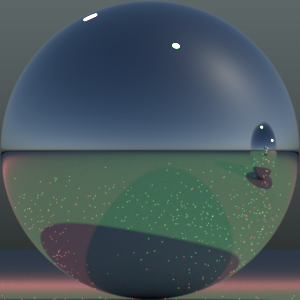
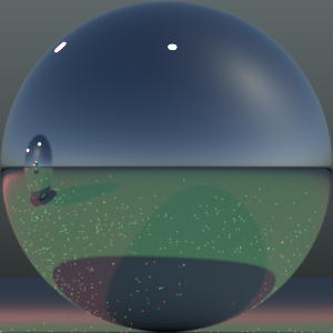
All the scenes were generated using the MITSUBA phisically-based rendering engine. Inside the scene I inserted two mirror balls to simulate the light probes and also inserted the light sources. The spheres were always at a good distance from the camera to simulate an orthographic projection.
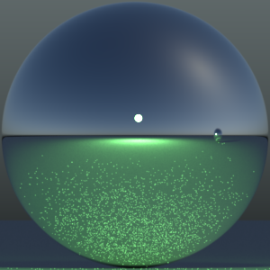
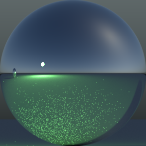
In the sequece one picture of each sphere was taken with a field of view that makes the mirror ball occupy the maximum space in the image without extrapolating its borders. A sky was used as environmental map. The last step was to take a third picture with a spherical camera which directly creates a latitude-longitude environment map. The scene is then rendered first using this environment map only and after with the light sources found with the stero light probe approach. Bellow a sequece of image showing this part of the pipeline.
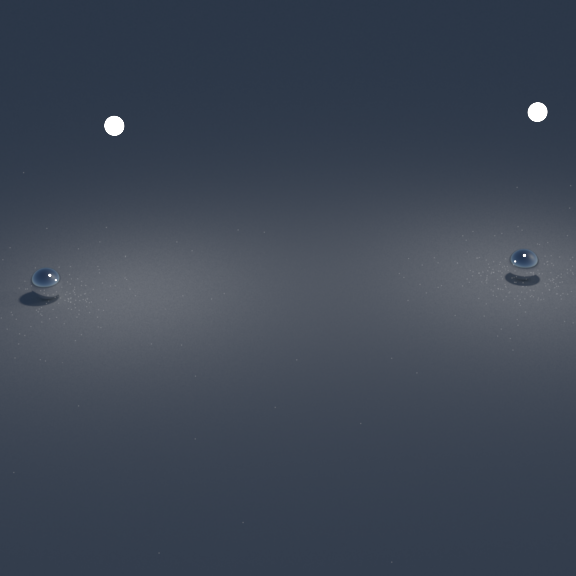
View of the scene with the mirror balls.
Part 2: Rectification of Spherical Images
After acquiring the images of the two spherical mirrors we have to find a correspondence between pixels and their position in space. Once we know which pixels from each spheres reflect the same point in the scene to the camera we can estimate a 3D location for the given point. But since the spheres were photographed from different locations/angles, we first need to find transform them to a common reference system that allows us to do such matching between pixels.
For this, the authors suggest an image rectification technique. Basically it works the following way: you have a point
p in space as shown in the picture bellow. Its reflection on each sphere is bounced towards the cameras $C_1$ and $C_2$, which is represented by the vectors $\vec{R_1}$ and $\vec{R_2}$. These two vectors lie on a particular plane, which passes throught the line that connects the two spheres (the dotted line and the line between the balls) and contains the point
p. Since we know this line (by having the position of spheres and cameras) we can use it as a guide to transform the pixels position to a common reference system. In this case, we use the latitude-longitude system with north and south pole as illustrated in the picture.
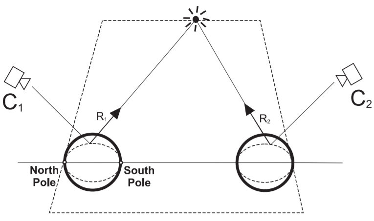
Schematization of reflection vectors.
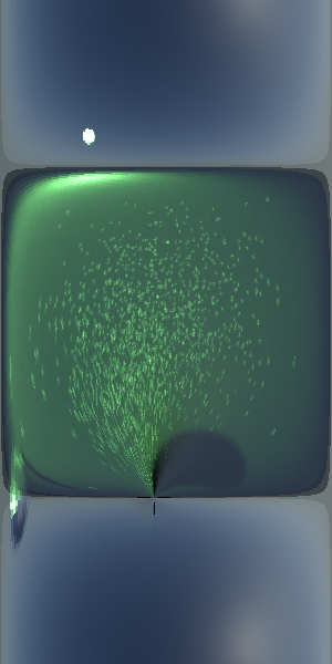
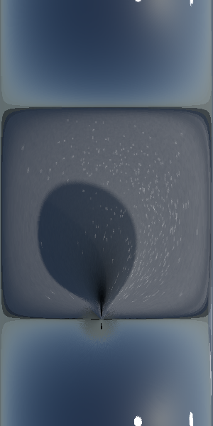
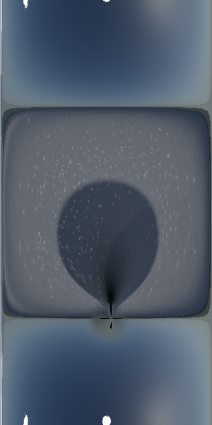
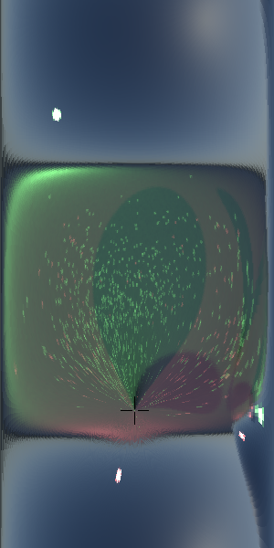
So the first pass is to transform the sphere into a equirectangular projection. For that we create an image where the rows correspond to the longitude $\theta$ (going from $0$ to $2\pi$) and columns to latitude $\phi$ (going from $-\pi/2$ to $\pi/2$). Each pair of ($\theta$,$\phi$) can be converted into $(x,y,z)$ with the following formulas:
$x = cos(\theta)$
$y = sin(\theta)cos(\phi)$
$z = -sin(\theta)sin(\phi)$
To get the rectified version of these points we just multiply by the view matrix ($\mathbb{R}^{4x4}$). Next we need to stablish a correspondence between 3D points and image pixels. For that we use the reflection equation, which is given by
$\vec{R} = \vec{I} - 2(\vec{I} \cdot \vec{N})\vec{N}$
where $\vec{I}$ is the vector indicating the direction the camera is looking at and $\vec{N}$ the normal of a 3D point, which is composed by the values of $(x,y,z)$ obtained from ($\theta$,$\phi$). We can obtain the values for $\vec{R}$ in the following way
$R_x = -2\vec{N}_z\vec{N}_x$
$R_y = -2\vec{N}_z\vec{N}_y$
$R_z = 1 - 2\vec{N}_z^2$
Assuming that the rays that goes from the sphere to the camera are parallel we can divide $R_x$ and $R_y$ by $R_z$ to eliminate their depth factor and we end up with the $x_c$ and $y_c$ coordinates. Then we just need to apply the projection matrix ($\mathbb{R}^{3x4}$) to these values and we get the $u$ and $v$ coordinates, which are the pixel coordinates.
Part 3: Correspondences Estimation
In order to estimate which light sources are the same in both spheres we only need to look at each line of the latlong representations. Once we find a high intensity value (which probably corresponds to a light source) in the same line for both pictures we assume it is a light source. To avoid getting multiple values for the same light source I detect transform the light sources into blobs and use its centroid as its location.
Part 4: Results
The first result consists of a single light source place near three statues. Since the light is really close to the objects the shadow should project with different orientations. But since the environment map does not handle this (since it represent an ideal distant illumination) the shadows end up being almost parallel. In contrast when the estimated light source is positioned in the place indicated by the algorithm we can see that the result looks much more coherent.
View of the scene with the mirror balls.
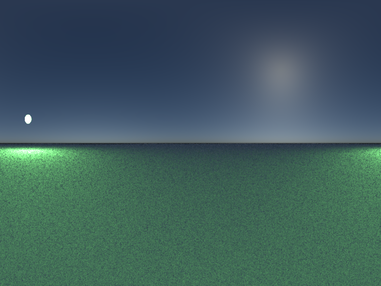
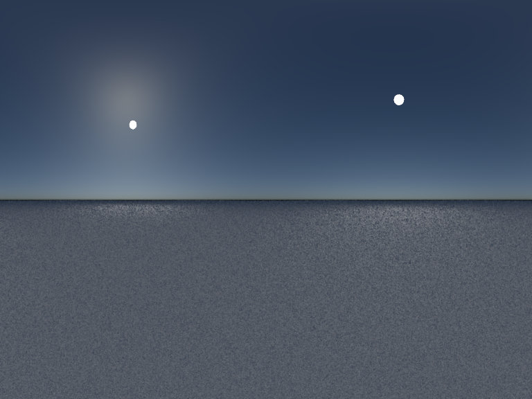
Environment map (one of the light sources is spread over the first rows of the image).
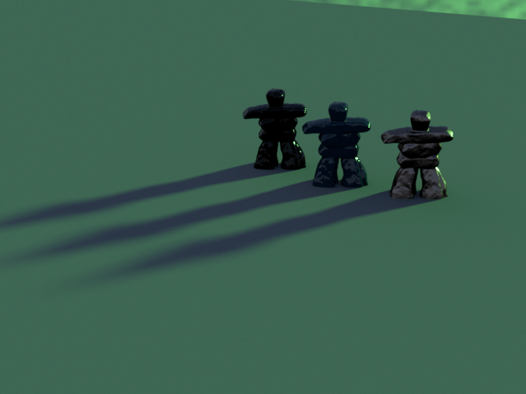
Image rendered with envmap.
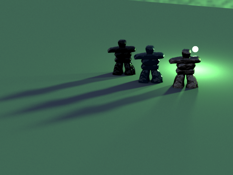
Image rendered with envmap and lights.
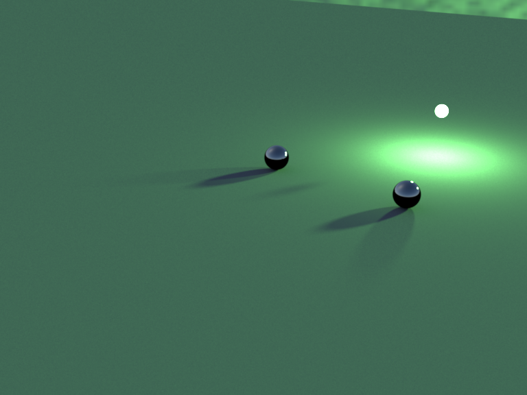
The second result is a composition of two lights situated at $[1, 1, 20]$ and $[-1.5, 1, 20]$. From the results it is possible to see that the shadow created by using the environment map only looks as coming from far away, thus projecting shadows similar in size to the objects. In contrast, the scene rendered with the estimated light sources (located at $[1.0029, 0.9426, 20.1647]$ and $[-1.5046, 0.9986, 19.9821]$) has more faithfull shadows according to the real light location.
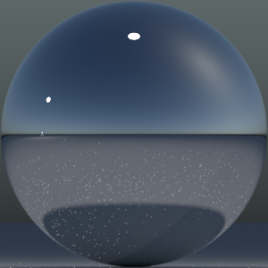
View of the scene with the mirror balls.
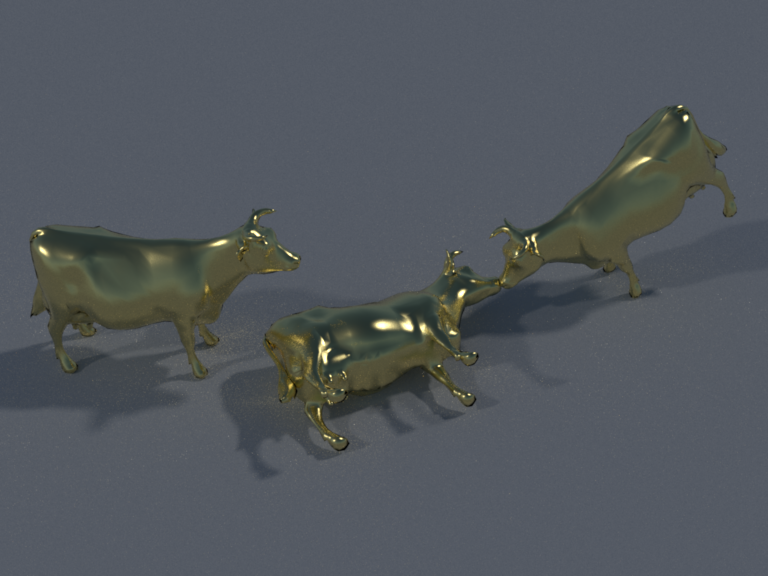
Image rendered with envmap.
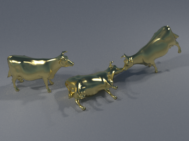
Image rendered with envmap and lights.
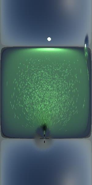
The third result is a composition of two spheres with different colors (green and blue). The first difference is the presence of the red color in the rendered image with the light positioned in their approximate location according to the algorithm output. Second is the shadows that again show a much more rich interactin between environment and objects: the cow to the right for example has a shadow that is being casted with a certain deformation that is in accordance with the position of light.
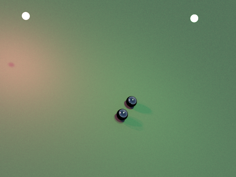
View of the scene with the mirror balls.
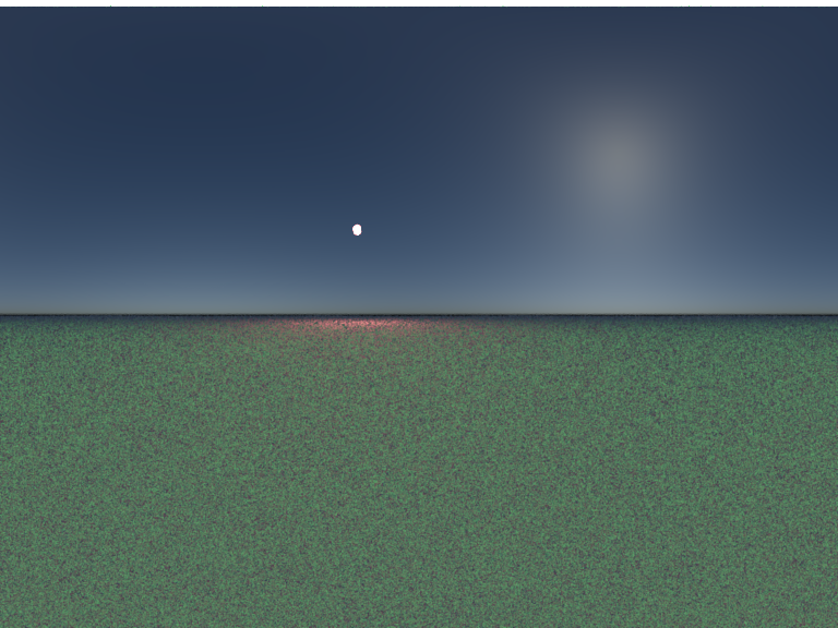
Environment map (one of the light sources is spread over the first rows of the image).
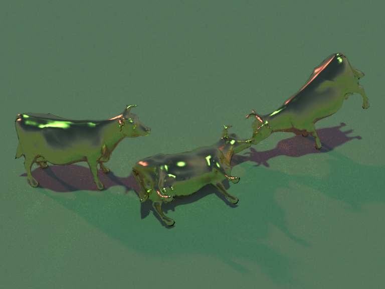
Image rendered with envmap.
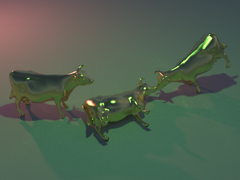
Image rendered with envmap and lights.