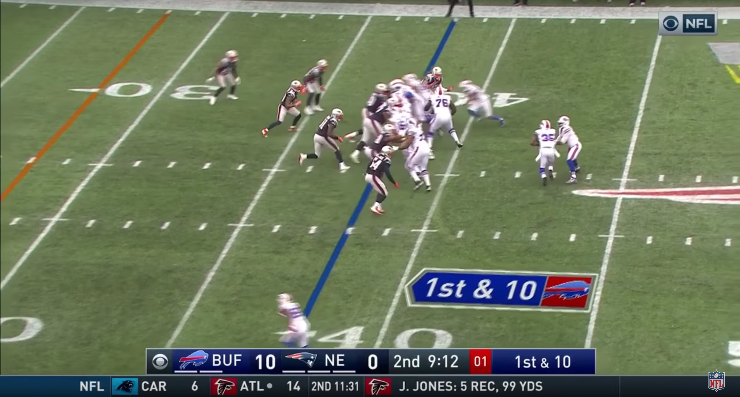
The virtual yellow became indispensable as soon as it appeared for the first time on television in the 90's. The first down line has forever change the way we look at football on television, adding crucial information about the distance the ball carrier need to get to in order to get a first down. However, in the non-professional industry, football coaches and managers have no way of virtually adding these important lines to their footage. With 1,085,272 highschool athletes in 2016, football is the no.1 participation sport in the U.S. Companies like Hudl have taken over the football footage management using web application. Having this kind of footage available on a backend server represent tremendous possibility to create automation process in order to add values to this footage with things such as first down and scrimmage lines.
Project description
The goal of the project is computing a virtual first down and scrimmage line using Python and OpenCV. The main approach is using reference points to compute homography matrix in order to convert frames between the actual footage and a real scale model of a football field (CFL in our case). After homography matrix are computed, lines are draw in the model and converted back in the actual footage using inverted homography matrix and HSV masks of the field.
Code
Code is available on Github
Homography calculation
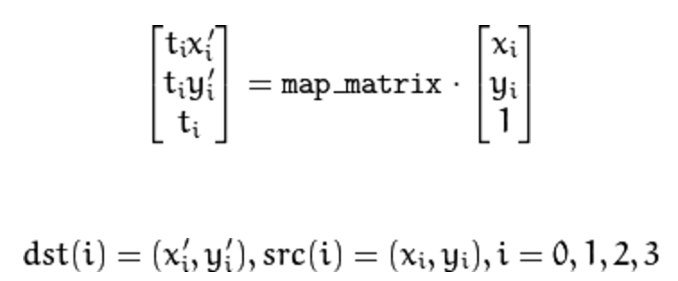
In order to draw the lines on the field, the first step is to compute the transformation matrix between the actual frame and the footbal field model. To find the homography matrix between the frame and the field model, the user need to gather 4 matching reference points in each of them.
Homography matrix calculation
Once the first homography is done by hand between the model and the first frame of the video, we can now find the homography of each following frame with the first frame. By dot multiplying them together we can retrieve the full homography of any frame to the model.
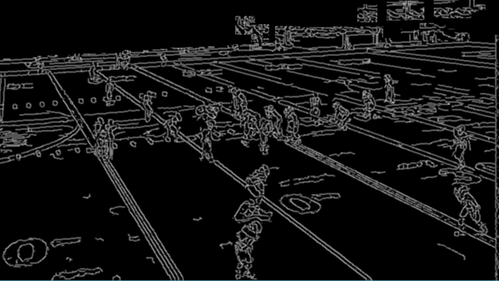
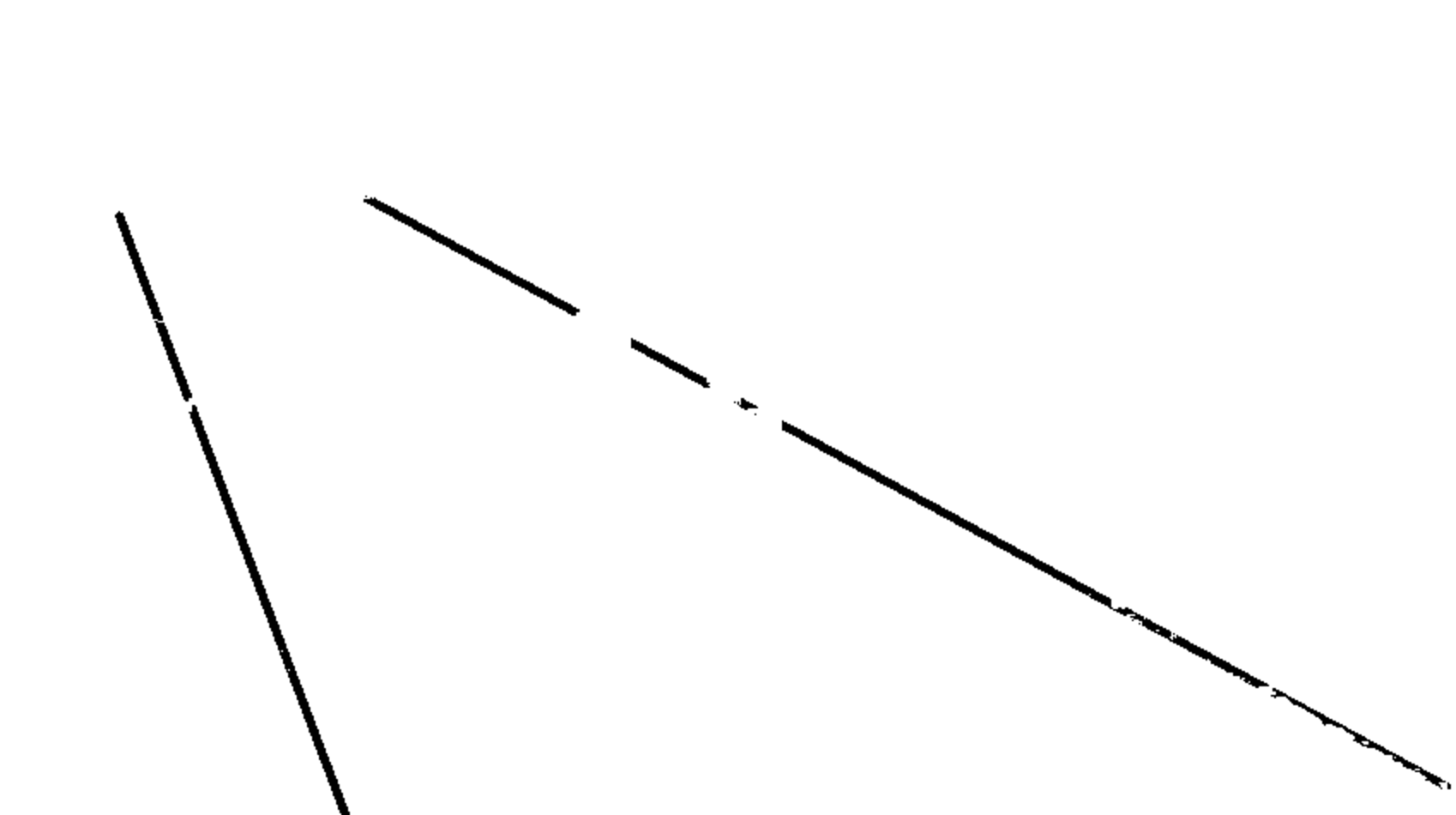
The first step to automize this process is to find the lines of the field of play. A simple feature matching of the frames will not give a good result because the moving players are often good features, but they are moving fast. To find the lines, we use a Canny detector with a Hough Probabilistique algorithm.
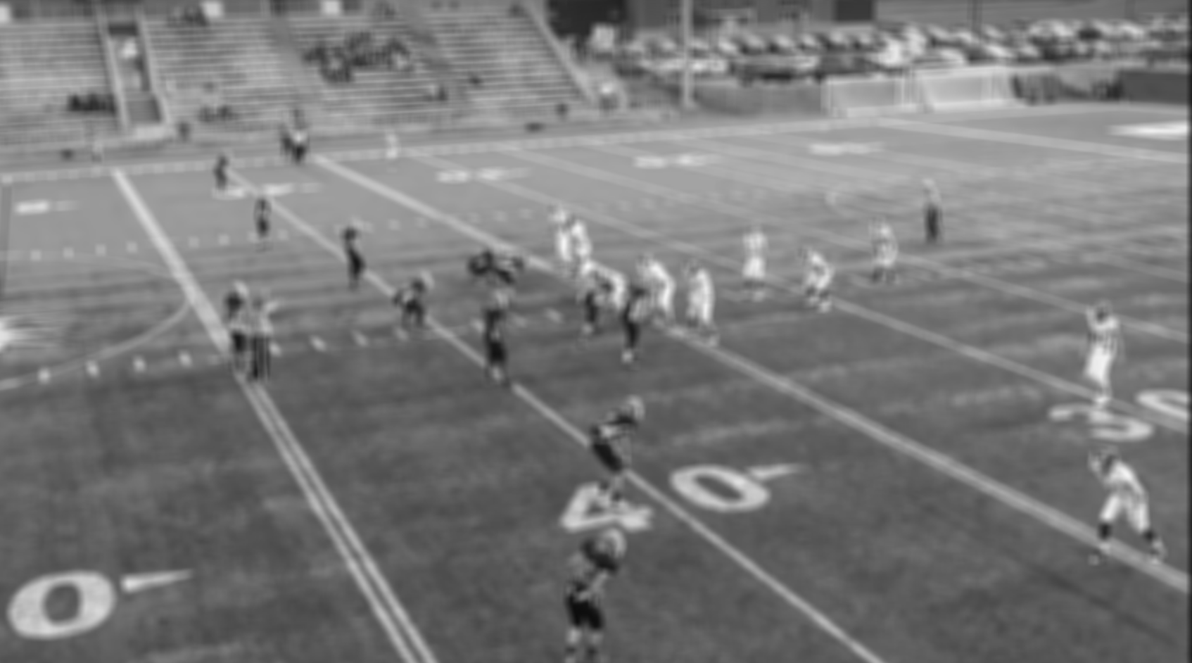
blurred image
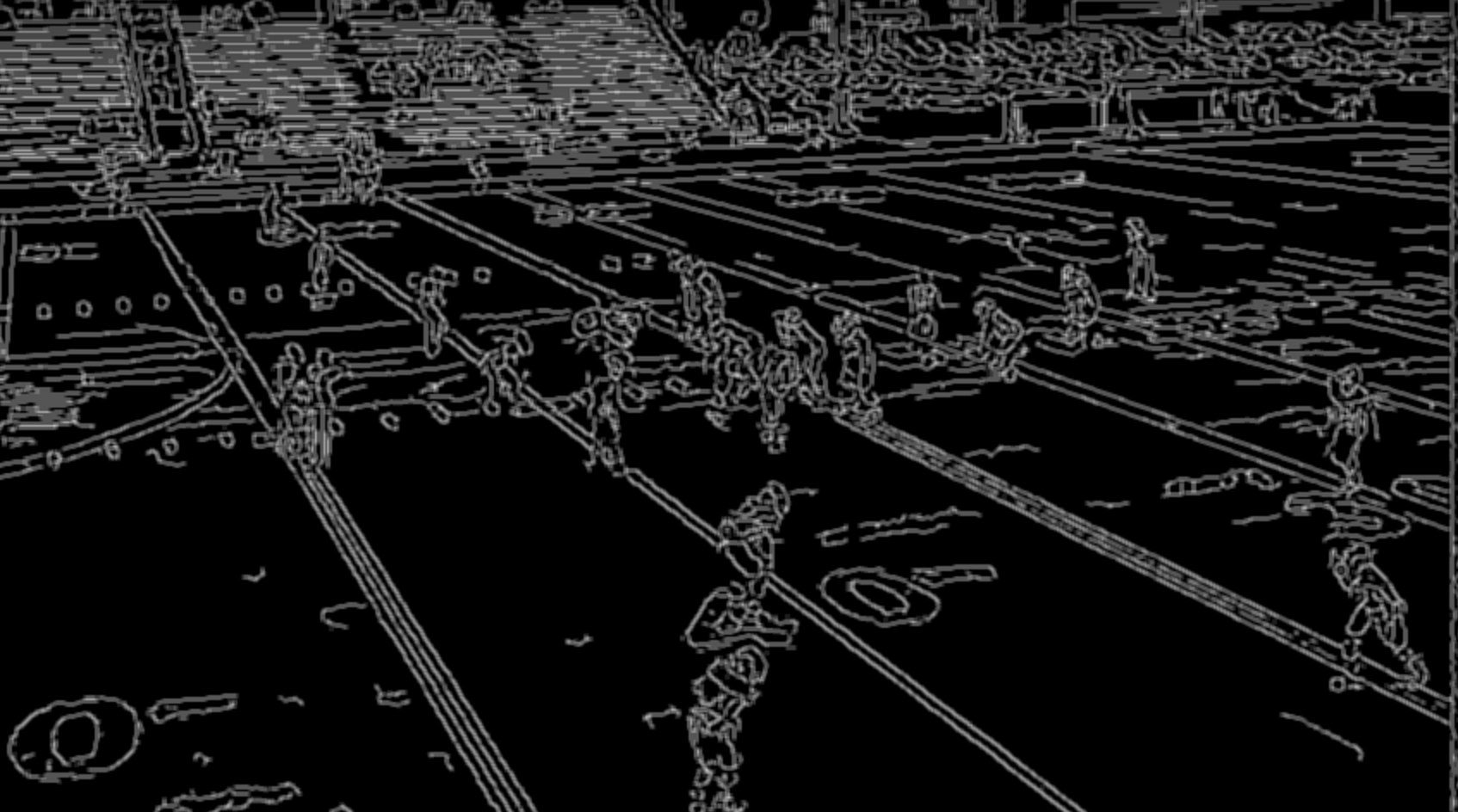
Canny
Canny cut
blurred image
Canny
Canny cut
We first blur the image to help the Canny detector to find smoother contours in the frame. We than use a Canny detector to find the contours. With of mask of the playing field (explained later) we can cut out un desired parts of the image. We can than find lines with the HoughLine detector algorithm. This algorithm will find all straight lines of a specific length minimum. We can then cluster the many lines into groups and find the median of the cluster. This will reveal all the lines of the field that are visible. Finaly we use a SSD to find the closest lines between to frames. We use at most 3 lines to do the Homography.
$$ \epsilon_{\hat{Y},Y} = \frac{1}{n} \sum_{i=1}^{n}(\hat{Y}_i - Y_i)^2 \quad ,$$Homography applied to original image in model
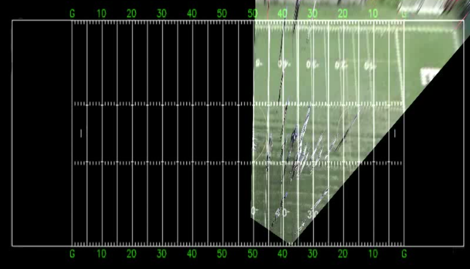
Once the homography matrix is computed, we select a point where the first down line should be located and a point for the scrimmage line. Next, the homography matrix is applied to both points to get the location of both clicked points in the field model. After that, the x coordinate of each point is taken and put with the y coordinates of both sidelines to create the extremities of the first down and scrimmage line in the field model.
Transformed points in field model
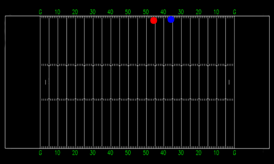
The inverted homography matrix is next applied to these lines extremities to retrieve the start and end point for each lines in the original image.
Line drawing
Now that the proper homography matrix has been calculated, the next step is to create masks in order to draw both lines on the field. To obtain realistic results, it's key to make sure that players and referees look like they are walking over the line. In order to achieve this, a window is created with HSV values sliders. This window allows to render the field mask with the current HSV values of the mask. Once the displayed mask is satisfying, two line masks are draw with the starting and ending points for each line calculated in the previous step.
HSV mask builder with sliders
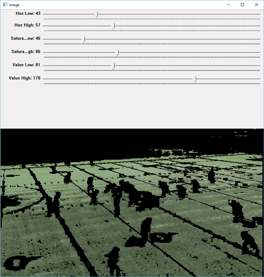
Generated field mask

Using different bitwise operations on masks, the inverted HSV field mask and the line mask are added together resulting in a line mask minus everything that is not the field such as players and referees. Next, those 2 lines are draw on the field.
Lines mask
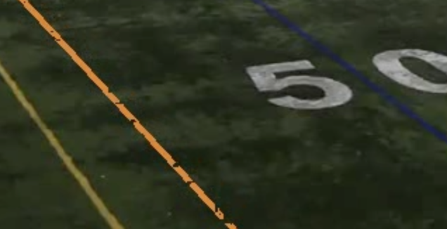
Generated image with first down and scrimmage lines
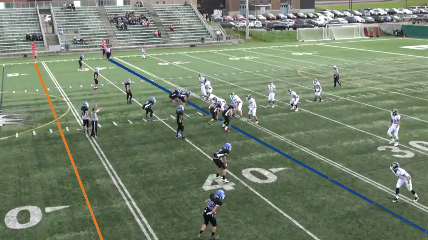
Results
Field 1 - Clip 1
Field 1 - Clip 2
Field 3 - Clip 2
Field 3 - Clip 3
Field 4 - Clip 5
Field 4 - Clip 6
As we can see in the different results, homography is often well computed in the first frames of the video when the camera hasn't move too much. As soon as the camera starts moving too much, homography calculation starts to fail and we lose the lines in the image. However, the line drawing in the footage is working pretty well. In the frames where the lines are draw, the masks seems to be well generated and the players and referees walk over it with no apparent problem. On certain fields, when the lighting is not very uniform, some problems occur due to the HSV mask and lines are sometimes not draw on certain spots on the field where they should be draw.
Line drawing problem on field with non-uniform lighting
References
[1] Timothy E. Lee, Automating NFL Film Study: Using Computer Vision to Analyze All-22 NFL Film, http://cvgl.stanford.edu/teaching/cs231a_winter1415/prev/projects/LeeTimothy.pdf