Laval University

Computational Photography

Homework 1 – Colorizing the Russian Empire

by Maxime Leclerc

February 1st 2015

Project description

Approach

Single scale algorithm results

Multiple scale algorithm results

Additional Prokudin-Gorskii results

Personal photos results

Problems encountered and solutions

Why are some images not aligned properly

Bells and whistles – Automatic contrast

Bells and whistles – Automatic border cropping

Project description

Sergei Mikhailovich Prokudin-Gorskii (1863-1944) was a Russian chemist and a pioneer in color photography. His photographic method was to divide the visible color spectrum into three channels using red, green and blue filters. This project aims to automatically combine these three channel colors into a single color image.

Red, green and blue filters. Source: uic.edu

Approach

The first thing the application does is to loop through all available JPG and TIF files. For each source file, we splits its content into three color channels: red, green and blue. We then automatically enhance the image's contrast. Please refer to the bell and whistles – automatic contrast section for additional details about this process.

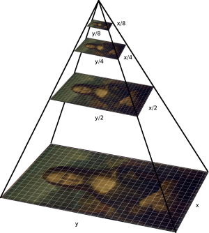
The next step is to align the three channels. We first check if the image is larger than 500 pixels. If that's the case, we recursively re-size the image half its size until we get an image smaller that is than 500 pixels. This multi-scale representation allows us to speed up computations on large images and is referred to as a pyramid representation.

Pyramid representation. Source: psu.edu

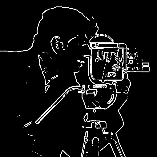
Before doing additional calculations, we simplify our color channels by transforming them into binary representations of the channels' edges. We use the Sobel method to perform this transformation. Please note that the Sobel method was used for this course by three students in 2014: Diane Fournier, Jingwei Cao and Tom Toulouse. It was also used by many Berkeley students for a Computational Photography course: Bilenko, Hall, Tang, etc. Using binary edge channels instead of gray scale channels improves our application's results in terms of quality and speed.

Sobel edge detection. Source: iastate.edu

For each re-sized or original image, we compute the sum of square differences (SSD) for different red-blue and green-blue channel alignments. The pyramid representation allows us to use a smaller search space for each image size. As a result, we compute the SSD for translations in the X and Y axes ranging only from -15 pixels to 15 pixels. In addition, we only compute the SSD for a 300 by 300 pixel region located around the center of each image. These two simplifications allow us to speed up computation, especially on large images.

The result of these calculations gives us the best alignment for the three color channels. We simply keep the alignment that has a minimum SSD - that is, our channel difference metric - over all the computed alignments. Note that when we switch from a small image to a larger image in our pyramid representation, we use the small image's alignment estimate as a starting point to find the best alignment for the larger image.

Once the original channels have been aligned, we then automatically crop the image's border. Please refer to the bell and whistles – automatic border cropping section for additional details about this process.

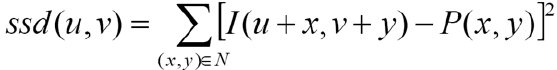
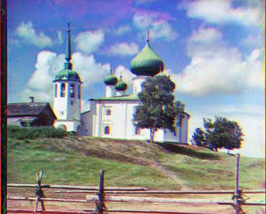
Single scale algorithm results

Calculated red offsets: X = 9, Y = -1.

Calculated green offsets: X = 4, Y = 1.

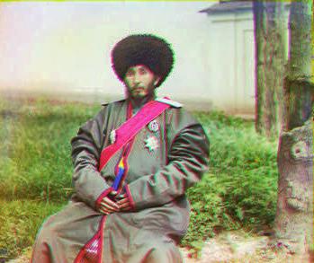
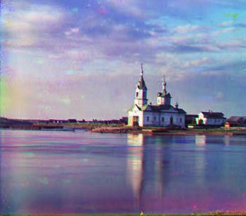
Calculated red offsets: X = 5, Y = 5.

Calculated green offsets: X = 2, Y = 3.

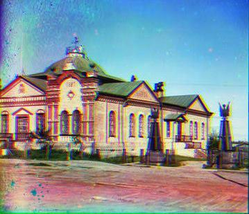
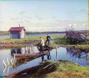
Calculated red offsets: X = 12, Y = 0.

Calculated green offsets: X = 6, Y = 1.

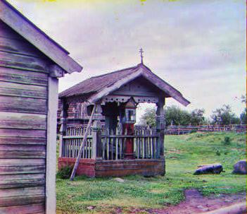
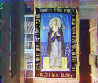
Calculated red offsets: X = 4, Y = 3.

Calculated green offsets: X = 2, Y = 2.

Calculated red offsets: X = 6, Y = 0.

Calculated green offsets: X = 2, Y = 0.

Calculated red offsets: X = 13, Y = -1.

Calculated green offsets: X = 1, Y = -1.

Calculated red offsets: X = 4, Y = 2.

Calculated green offsets: X = 1, Y = 1.

Calculated red offsets: X = 12, Y = 1.

Calculated green offsets: X = 5, Y = 1.

Calculated red offsets: X = 14, Y = 4.

Calculated green offsets: X = 6, Y = 2.

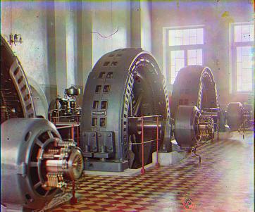
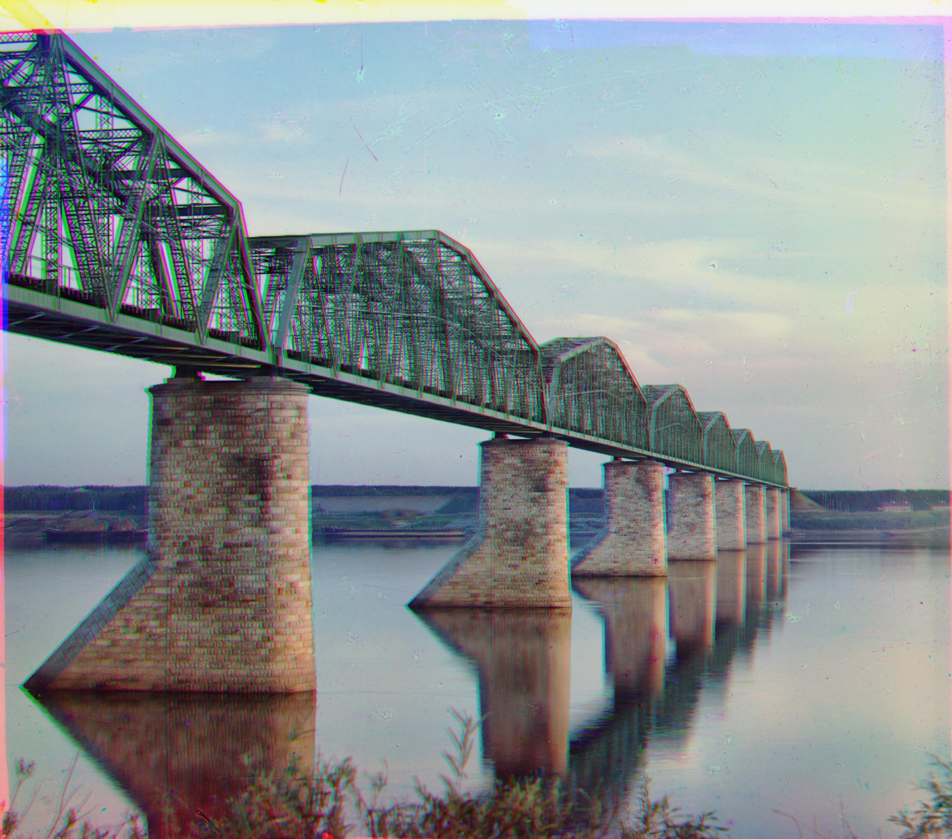
Multiple scale algorithm results

   Calculated red offsets: X = 87, Y = 38.

   Calculated green offsets: X = 35, Y = 19.

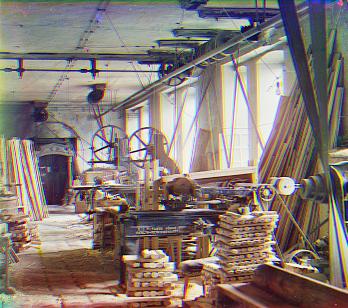
   Calculated red offsets: X = 108, Y = 68.

   Calculated green offsets: X = 49, Y = 51.

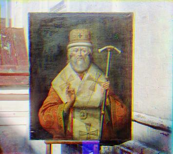
   Calculated red offsets: X = 52, Y = 38.

   Calculated green offsets: X = 34, Y = 25.

   Calculated red offsets: X = 85, Y = 32.

   Calculated green offsets: X = 42, Y = 6.

Calculated red offsets: X = 48, Y = 13.

Calculated green offsets: X = 14, Y = 5.

Calculated red offsets: X = 123, Y = 34.

Calculated green offsets: X = 56, Y = 25.

Calculated red offsets: X = 43, Y = 6.

Calculated green offsets: X = 16, Y = 5.

Calculated red offsets: X = 12, Y = 20.

Calculated green offsets: X = -15, Y = 10.

Calculated red offsets: X = 71, Y = 34.

Calculated green offsets: X = 23, Y = 20.

Additional Prokudin-Gorskii results

Calculated red offsets: X = 14, Y = 5.

Calculated green offsets: X = 6, Y = 3.

Calculated red offsets: X = 5, Y = 5.

Calculated green offsets: X = 2, Y = 3.

Calculated red offsets: X = 11, Y = 3.

Calculated green offsets: X = 5, Y = 2.

Calculated red offsets: X = 13, Y = 4.

Calculated green offsets: X = 6, Y = 3.

Calculated red offsets: X = 10, Y = -4.

Calculated green offsets: X = 5, Y = -1.

Calculated red offsets: X = 69, Y = 8.

Calculated green offsets: X = 13, Y = -4.

Calculated red offsets: X = 119, Y = -15.

Calculated green offsets: X = 53, Y = -4.

Calculated red offsets: X = 152, Y = -6.

Calculated green offsets: X = 39, Y = -1.

Calculated red offsets: X = 129, Y = 25.

Calculated green offsets: X = 59, Y = 14.

Calculated red offsets: X = 113, Y = -24.

Calculated green offsets: X = 43, Y = -9.

Personal photos results

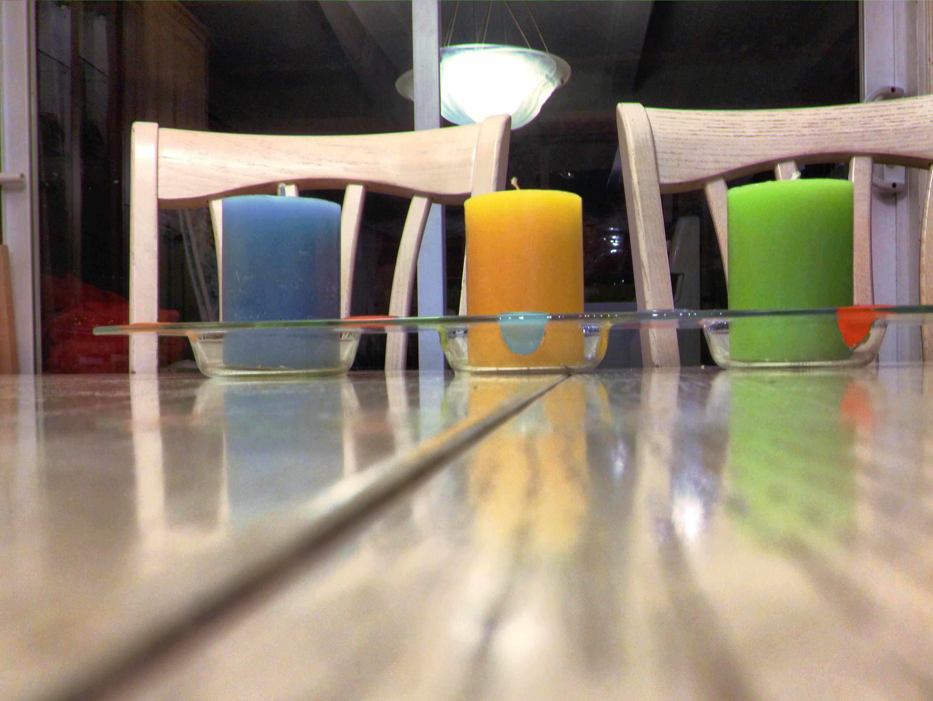
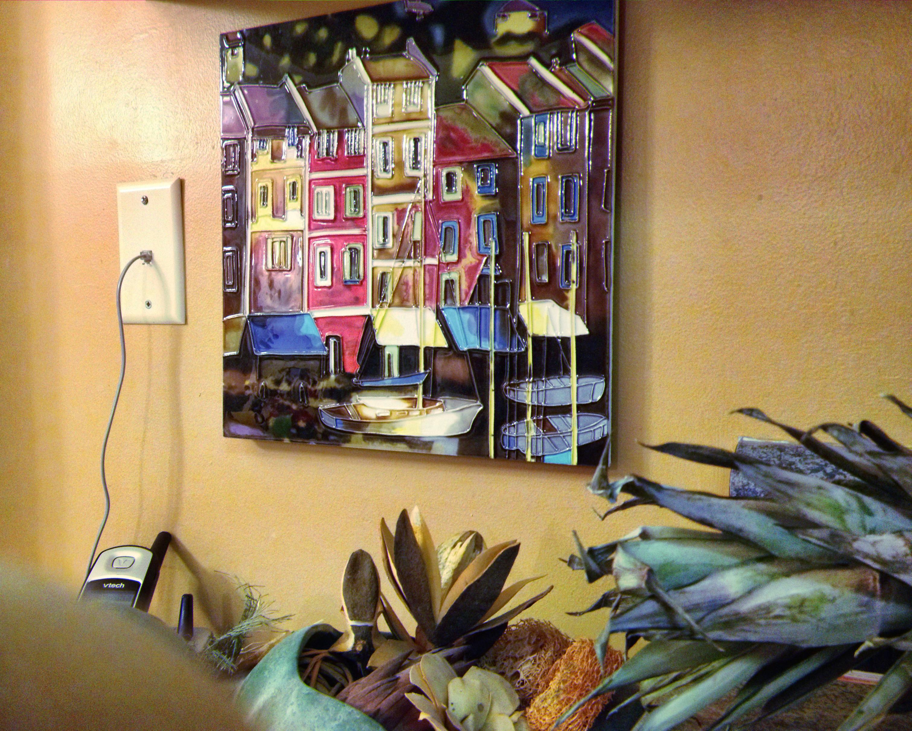
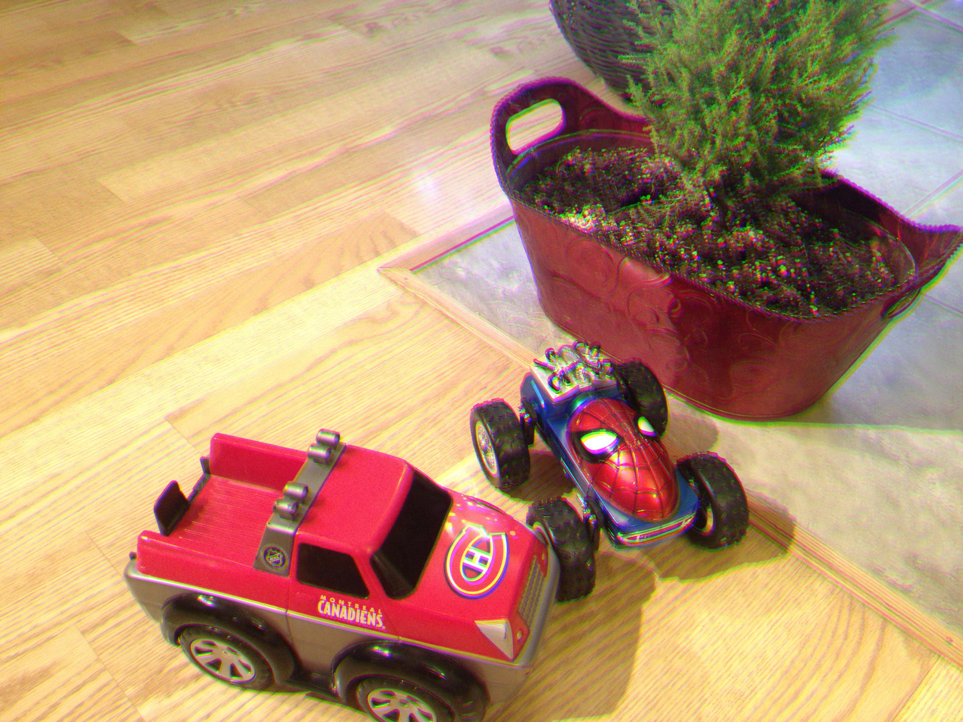
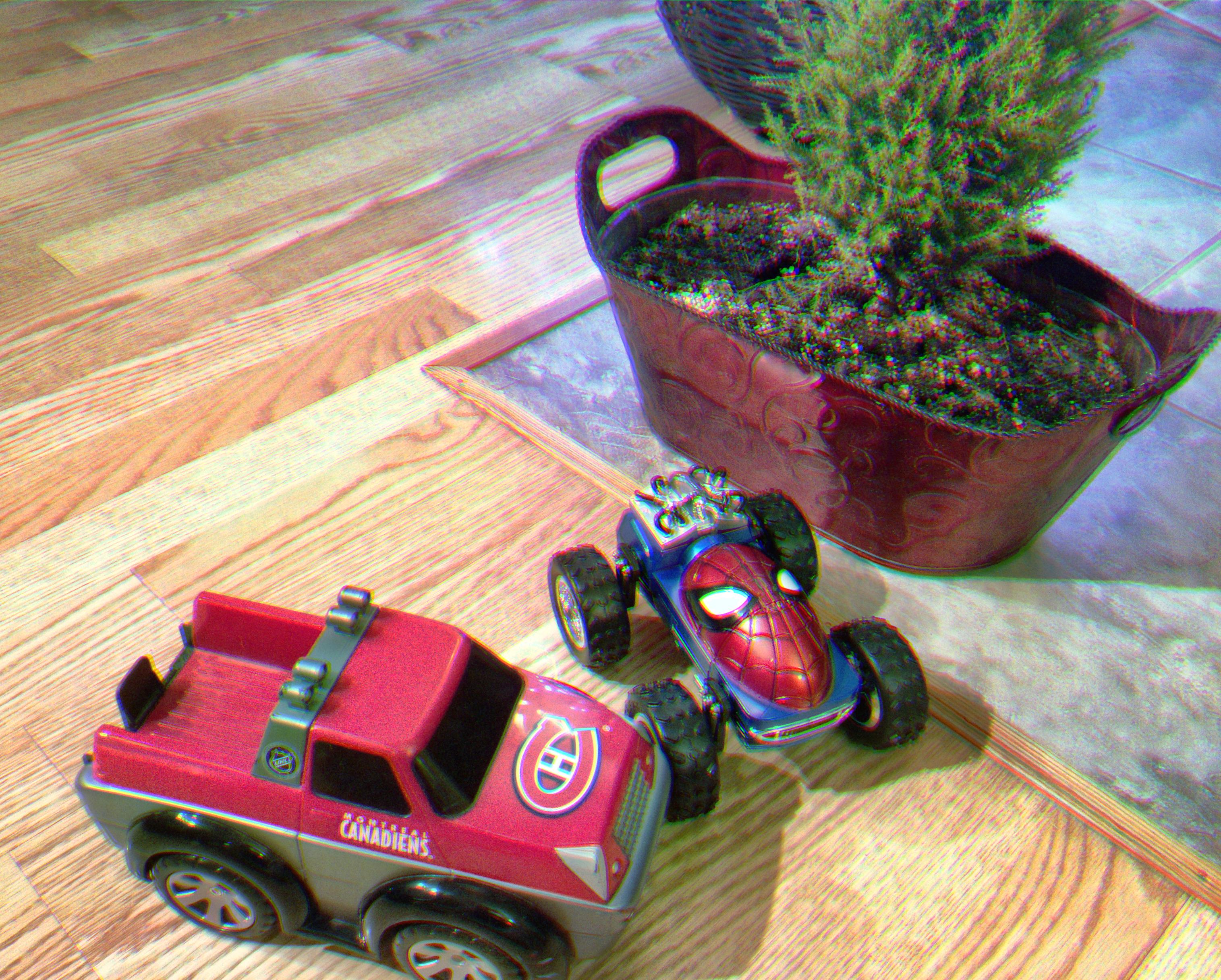
We tested out algorithms on our own photos. As expected, the best results we get are when there is no movement in the scene and when the camera does not move. Here are some before and after images:

Before

original-candles(1).jpg.jpg

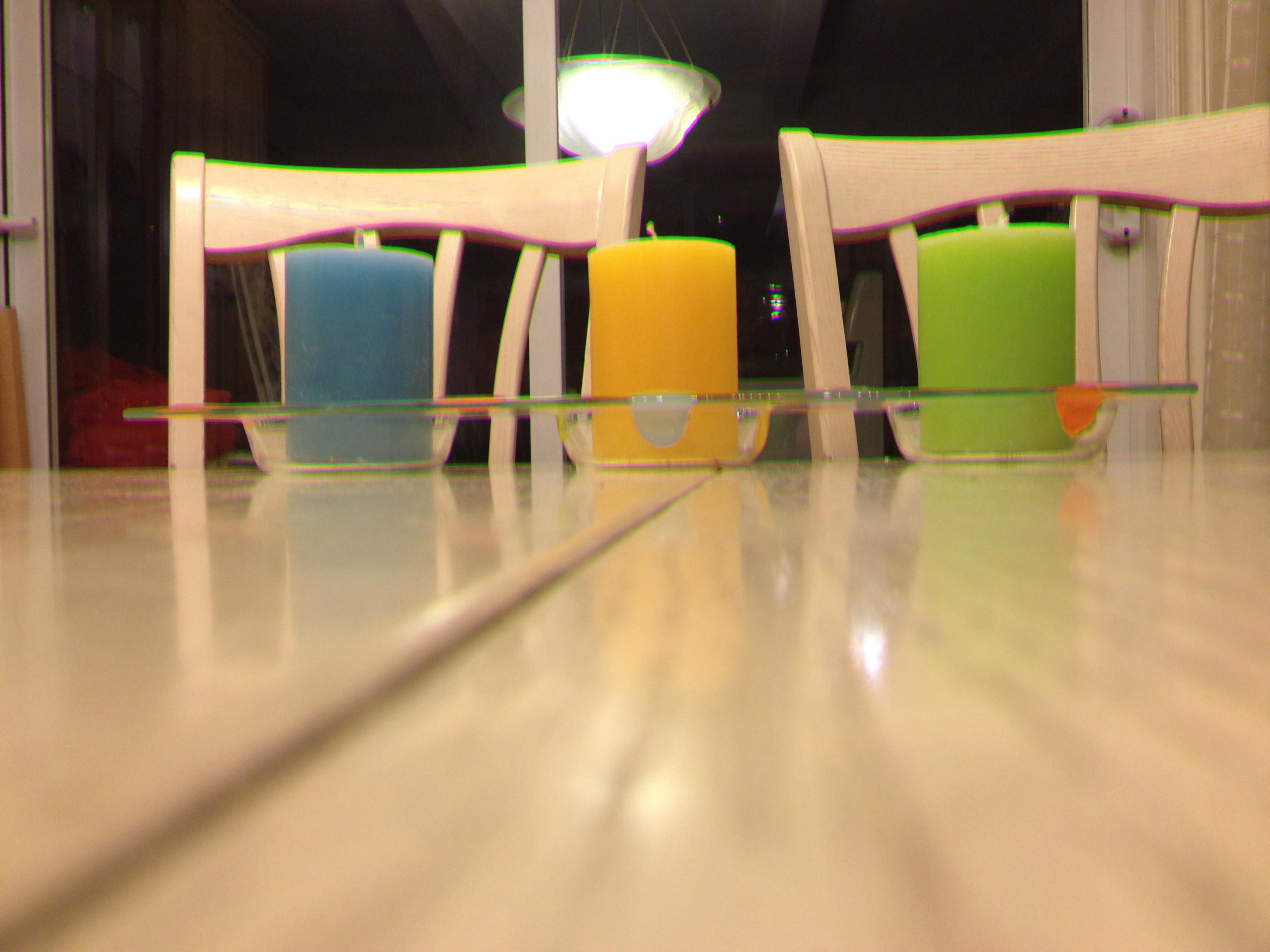
After

Calculated red offsets: X = 4, Y = 1.

Calculated green offsets: X = 11, Y = 1.

Before

original-wall(1).jpg.jpg

After

Calculated red offsets: X = 24, Y = -1.

Calculated green offsets: X = 27, Y = -1.

Before

original-toys(1).jpg.jpg

After

Calculated red offsets: X = 12, Y = 2.

Calculated green offsets: X = 13, Y = 1.

Problems encountered and solutions

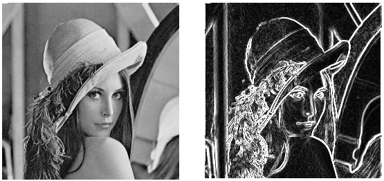
The first problem we encountered was that a simple color channel comparison did not give good alignment results. This explains why we decided to transform the color channels into edge images with the Sobel method. Using this simplified representation gives much better alignment results than the results we had with raw images.

Sobel edge detection. Source: umn.edu

Next, we had to do some trial and error when we developed the automatic contrast operation. We had to chose among many different contrast transformations. We had poor results with some transformations and decided to pick a hybrid solution that combined the best results in a single image. See the section below for details about the final solution. Finally, we had to tweak a few threshold values when we created the automatic border cropping. See the last section for additional details on this process.

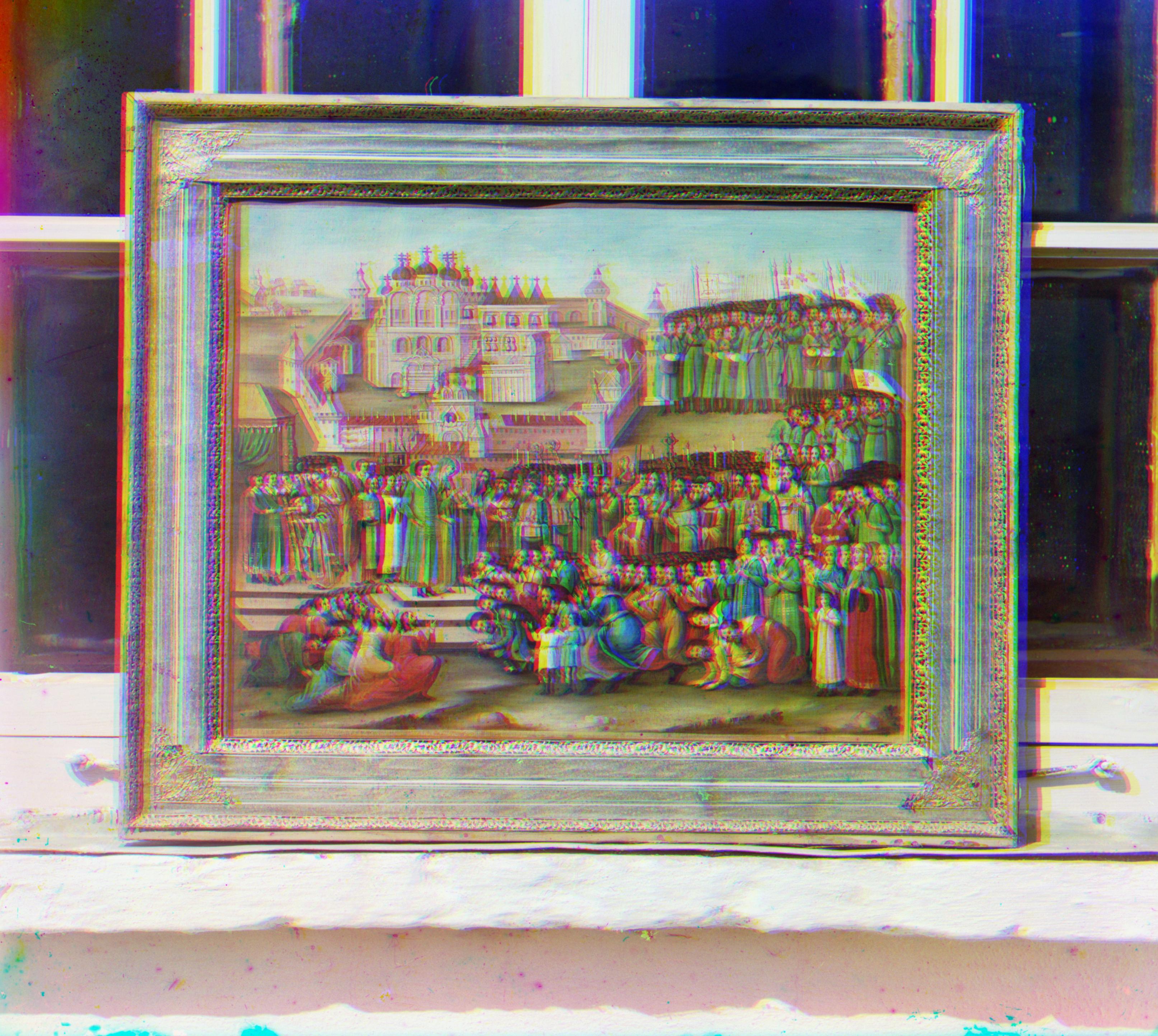
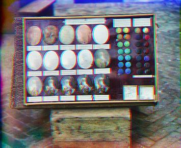
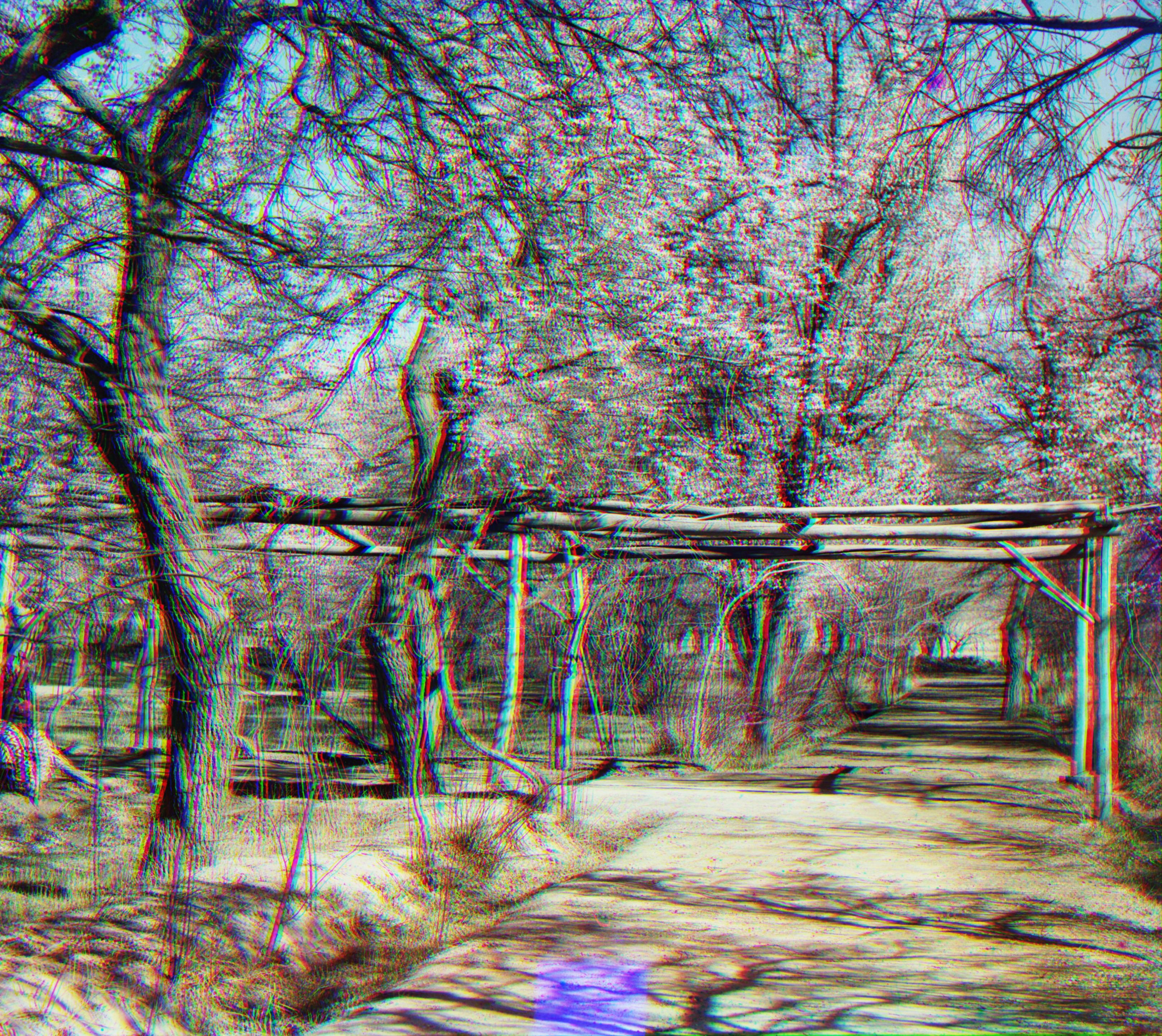
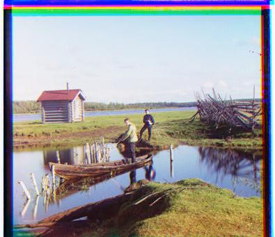
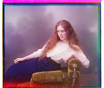
Why are some images not aligned properly

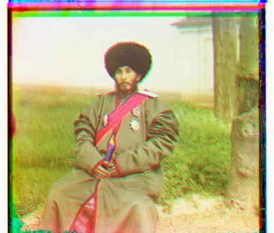
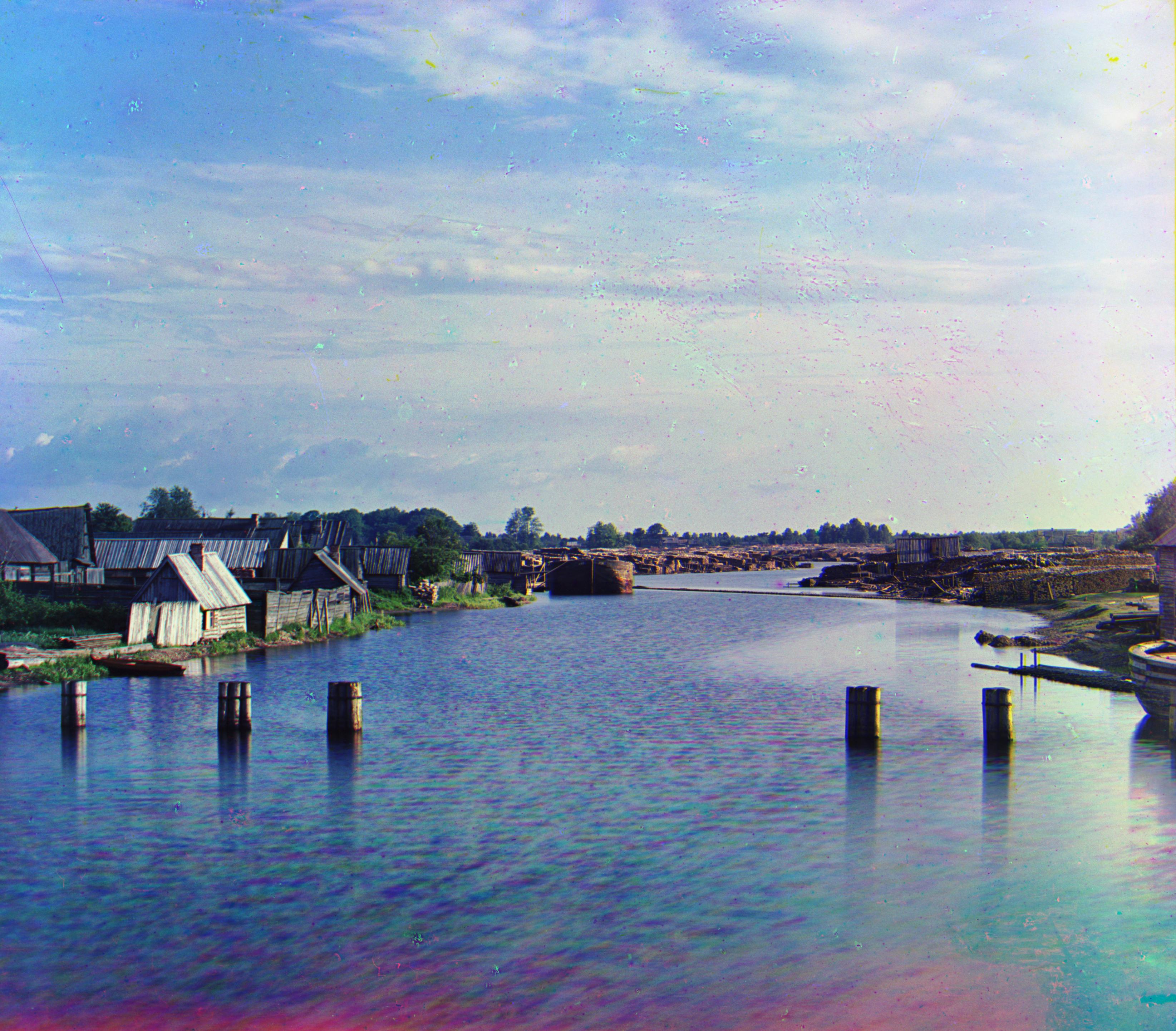
We can see that our algorithms are not entirely robust for all images. For example, the following image doesn't seem to be aligned properly:

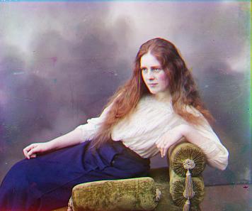
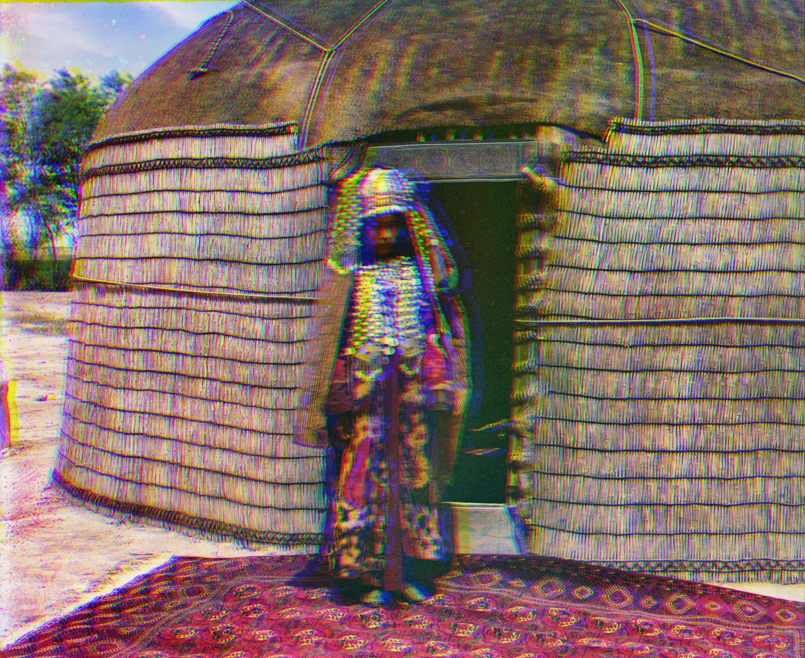
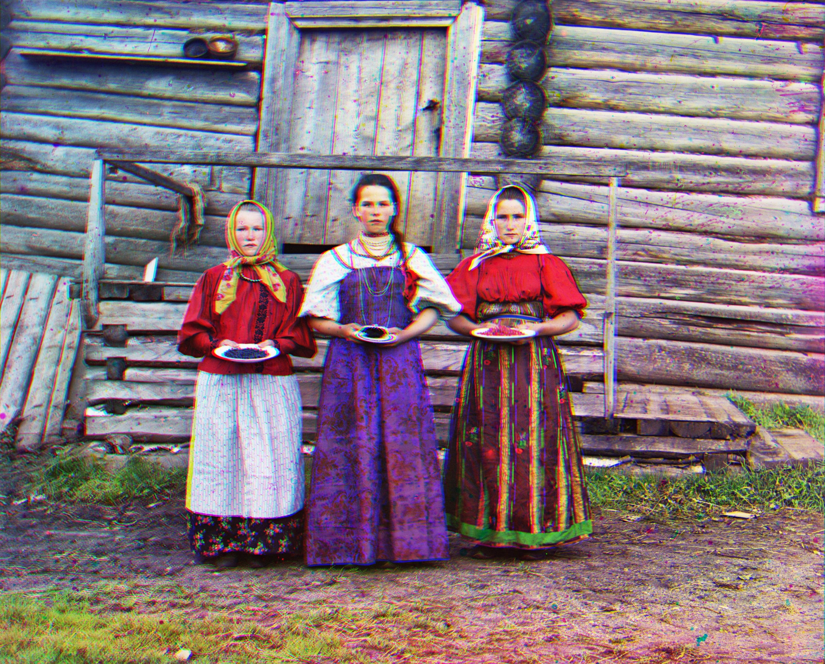
One possible explanation could be that the woman in the middle as well as the trees and the clouds located on the left side moved while the photographer was changing the color filters. We also see some hard to avoid human movement in the next photo featuring three young women. Most of the image seems to be correctly aligned except for the region around the young women:

Bells and whistles – Automatic contrast

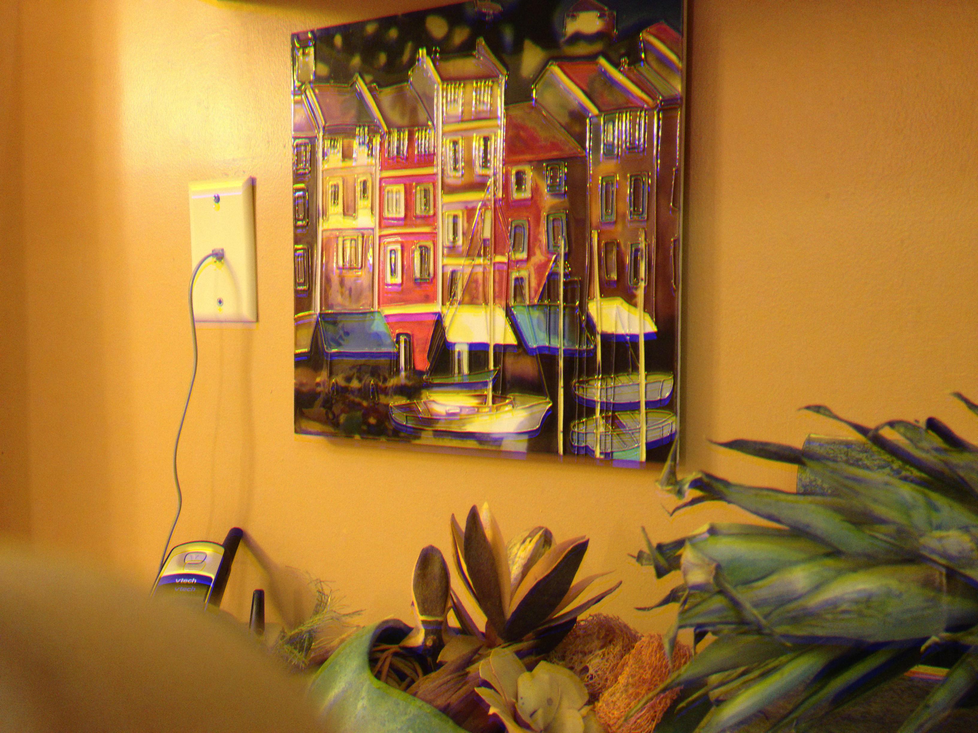
To automatically improve image contrast, we use a simple histogram equalization and a contrast-limited adaptive histogram equalization (CLAHE). This gives us two new image versions in addition to the original version. After some testing, we found that each of these three image versions contributed interesting visual information not necessarily present in the other two image versions. As a result, we decided to average the original image with these two histogram equalizations in order to benefit from all three versions' visual information content.

Here are some before and after images:

Before automatic contrast

After automatic contrast

The left image above had too much yellow in it. The image to the right corrected this issue.

Before

After

We could barely see the clouds in the left image above. However, the clouds are now visible in image to the right.

Before

After

The first image had too much red in it. The second image seems more realistic.

Bells and whistles – Automatic border cropping

    For the automatic border cropping process, we first compute the difference between each channel. We then sum these differences across all the image's rows and columns. This gives us two vectors: a vector containing the sum of channel differences for each horizontal row and one containing the sum of channel differences for each vertical column. Here's a short pseudo code example:

    borderDiff = channelDifference( Red, Green ) + channelDifference( Red, Blue )
        + channelDifference( Blue, Green );

    sumBorderX = sumOverX( borderDiff );
    sumBorderY = sumOverY( borderDiff );

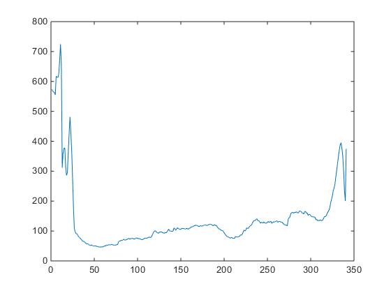
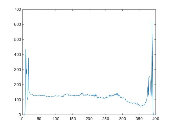
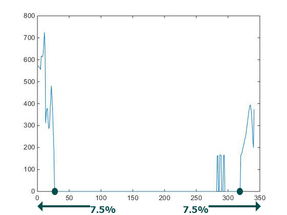
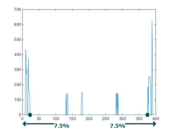
    Please note that a similar cropping method was used in 2014 by Peng Xue for a Berkeley Computational Photography course. In adition, Tom Toulouse also used a similar method for this course in 2014. Here are sample plots for a given image of these two summed difference vectors - one summed horizontally, the other summed vertically.

    From these plots, we can clearly see that the summed difference is higher in the first and last few rows as well as in the first and last few columns.

Channel difference summed over X

Channel difference summed over Y

Next, to automate the cropping process, we need to chose thresholds that work well for most images. We have two goals here: 1) Preserve interesting visual information and 2) Cut the image where it is inconsistent.

Preserve interesting visual information

One threshold we implemented is used to limit the maximum region we allow to be cropped. After some tweaking, a value that seems to work well is to limit the cropping to a portion of 7.5% of the total image size for each cropping region (at the top, bottom, left and right). This threshold ensures that we don't crop the image too much and that we don't lose interesting visual information.

Cut the image where it is inconsistent

A difference value above the mean value indicates that the region is dissimilar across the three channels. After some tweaking, we found that using 115% of the mean value was a better threshold than using the actual mean value when we crop the test images. In other words, we want to crop a border region when this region has a channel difference metric higher than 115% times the metric mean.

Original border difference summed over X

Selected X values greater than 115% x mean value

The arrows and circles at the bottom represent approximations of the search operations and results.

Original border difference summed over Y

Selected Y values greater than 115% x the mean value

The arrows and circles at the bottom represent approximations of the search operations and results.

With that in mind, we crop the image using the rightmost above average value. Remember that we limit ourselves to the region corresponding to the first 7.5% portion of each vector. We also crop the image using the leftmost above average value. Again, we limit ourselves to the region corresponding to the last 7.5% portion of each summed difference vector.

    maxCropRegion = 7.5%;

    firstCroppedX = findFirstVectorElement( vectorSearched = selectedXValues,
        findFirstVectorElement > 0, searchDirection = 'fromRightToLeft',
        startAt = ( lengthVectorX * maxCropRegion ) );

Here are some before and after images:

Before cropping