Final Project
Indicator Mineral in Hyperspectral imaging
by Saeed Sojasi
Goal of Project
In general, the hyperspectral mineral finding has been defined in the hyperspectral remote sensing and satellite imageries.
However, the considering that some mineral are valuable and cannot be found in the larger forms the geological sampling seemingly essential
and a quick automatic mineral identification looks required. The goal of the project is automatic identification of the mineral grains
through hyperspectral imageries and data-mining procedure. The information required for identification of the minerals are essentially follows
the geological information and follow the mineral spectroscopy data for each mineral grains depend on the size,
angle and band of wavelength which acquisition is done (will be explained in future sections).
We put g=ln(f -1). Then we have:
Hyperspectral imaging
Hyperspectral images contain all electromagnetic spectrum and process information from across the electromagnetic spectrum.
Hyperspectral images have many applications such as: agriculture, resource management, mineral exploration, and environmental monitoring.
Imaging spectrometers produce hyperspectral images.
This tool has some complex sensors. [1]
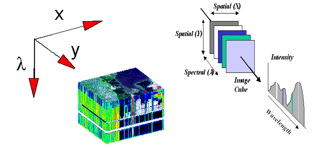
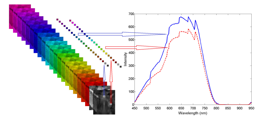
In hyperspectral images we have a image cube instead of two dimensional image. It has two spatial dimension and one spectral dimension.
for this project, we are going to reach intensity-wavelength curve.
Electromagnetic Wavelength
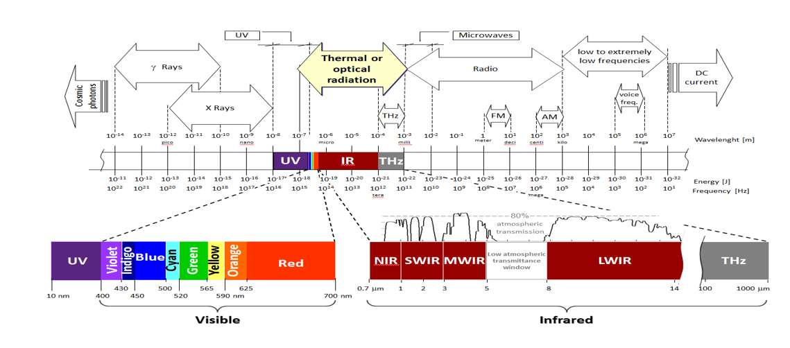
For this project we works on Infrared and visible bands.
There are general spectral ranges for ultraviolet, visible, and infrared:
Ultraviolet (UV): 0.001 to 0.4 µm
Visible: 0.4 to 0.7 µm
Near-infrared (NIR): 0.7 to 3 µm
Mid-infrared (MIR): 3 to 30 µm
Far infrared (FIR): 30 µm to 1 mm
For remote sensing these ranges are different. These ranges are not standard, just use for remote sensing:
Visible Near Infrared (VNIR): 0.4 to 1 µm
Short wave Infrared (SWIR): 1 to 2.5 µm
Mid wave Infrared (MWIR): 2.5 to 3 µm
All pure minerals have a spectral signature like fingerprints in visible and infrared bands. The signature of Quartz is shown as below [2]:
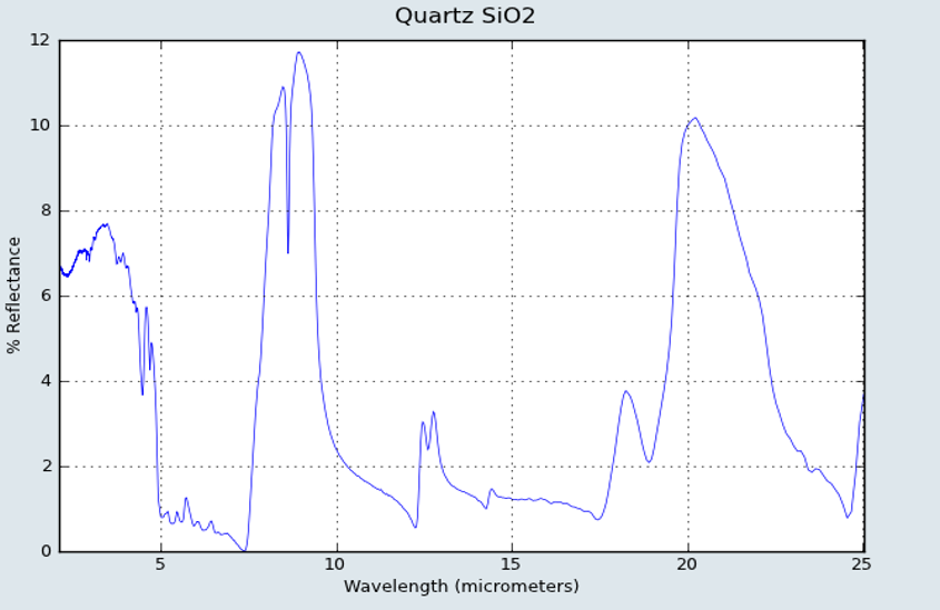
This example shows the signature of Quartz from 0µm to 25µm.
We want to detect of pure sample`s reflectance in electromagnetic wavelength (visible and infrared).
After that, by using spectral signature of pure sample we are going to detect synthetic materials.
In real world we have synthetic minerals instead of pure minerals. Each part of synthetic materials has different reflectance.
This difference depends on type of material in that part.
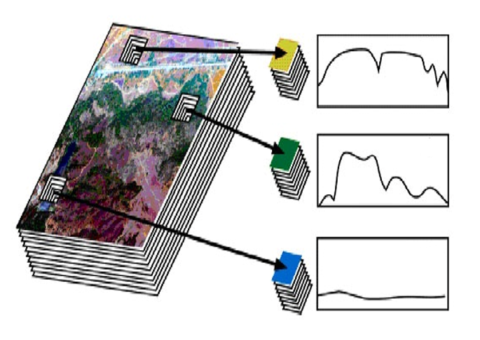
We can see an example of synthetic result of minerals in visible and mid-infrared bands:
In spectroscopy reflectance of light from the materials surface is measured. The ratio of reflectance is a function of wavelength.
Reflectance is vary in different wavelength. After the measure of reflectance in different wavelength,
we compare reflectance curve in electromagnetic bands with signature of pure sample from NASA data set.
We can detect minerals type by comparing of reflectance curve in visible and infrared band by our data set. Minerals are a inorganic materials.
Chemical composition and crystalline structure control of spectral curve.
There are several libraries of reflectance spectral that available for public use.
ASTER spectral library has been made by NASA. Advance Spaceborne Thermal Emission and Reflection Radiometer (ASTER).
speclib.jpl.nasa.gov
USGS spectral library is another available library for public use. The United State Geological Survey Spectroscopy (USGS).
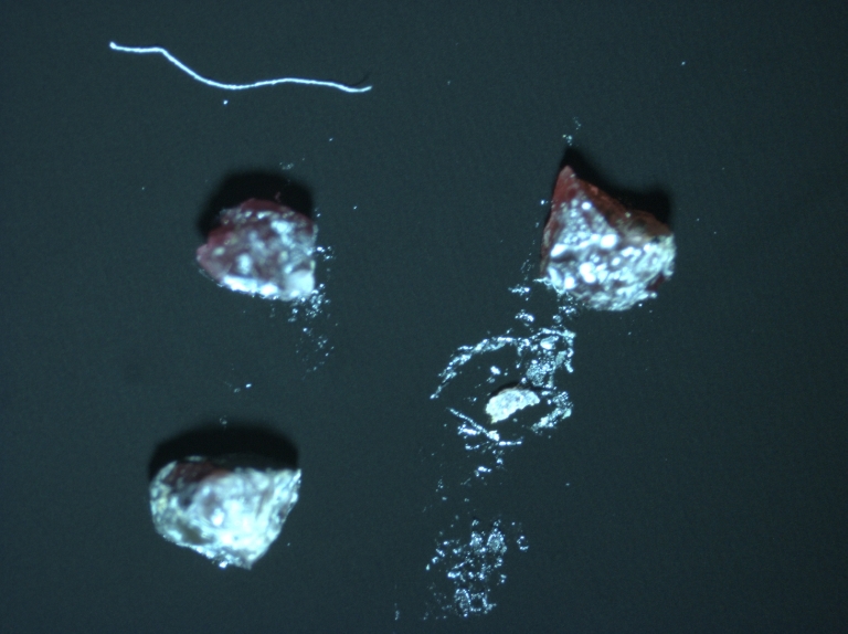
Hyperspectral camera (Telops Inc. Camera)
Hyp-Cam Lw is a lightweight and compact imaging radiometric spectrometer. It works with Fourier Transformer Infrared (FT-IR) sensor.
FT-IR allows us to identify either gas or solid from distance up to 5 kilometers.
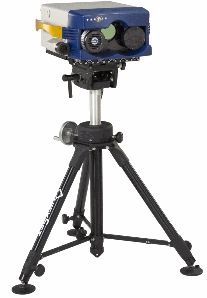
Camera characteristics
• NESR = noise equivalent spectral radiance
• It can work at Operating Temperature from -10oC to +45oC
• Weight 31 kg
Take Photo
Measurement of the same sample repeated and we get multiple data cubes.
This data cube is an image 64 × 20 pixels and spectral resolution is 6.2 cm -1.
This camera captured 20 frames in 30 seconds. This procedure repeats 3 runs and finally we get 60 frames.
2 frames remove. Finally, we have 58 frames.
Camera Calibration
It has two internal calibration blackbodies. Cold and hot BB temperature set at 15oC and 65oC and
ambient temperature set at 22oC.
BB spectral radiance determine using the Planck function. [4]
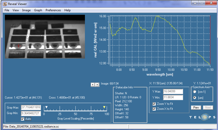
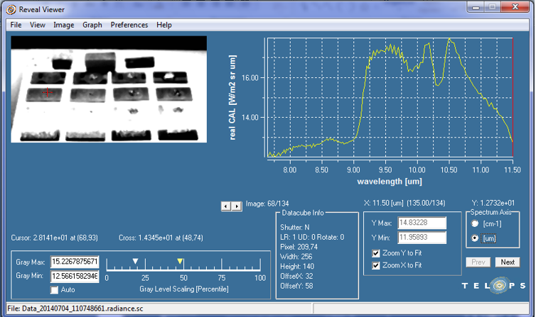
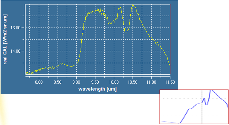
Result of TELOPS
By the TELOPS software (Reveal Viewer) I did these tests. This camera takes photo in 134 bands. It means we have one image in each 30 nm.
Electromagnetic Wavelength: From 7700 nm to 11800 nm
Hyperspectral bands: 134
((11800-7700))/134 = 30.59 ≈ 30 nm
In every 30 nm we have one image
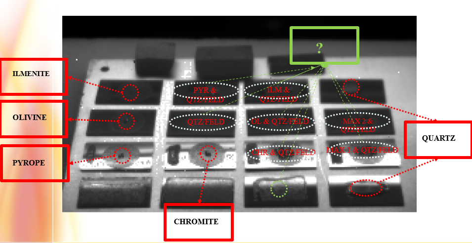
Image from [9]:
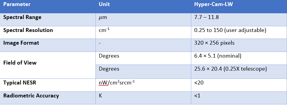
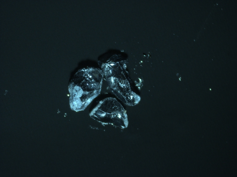
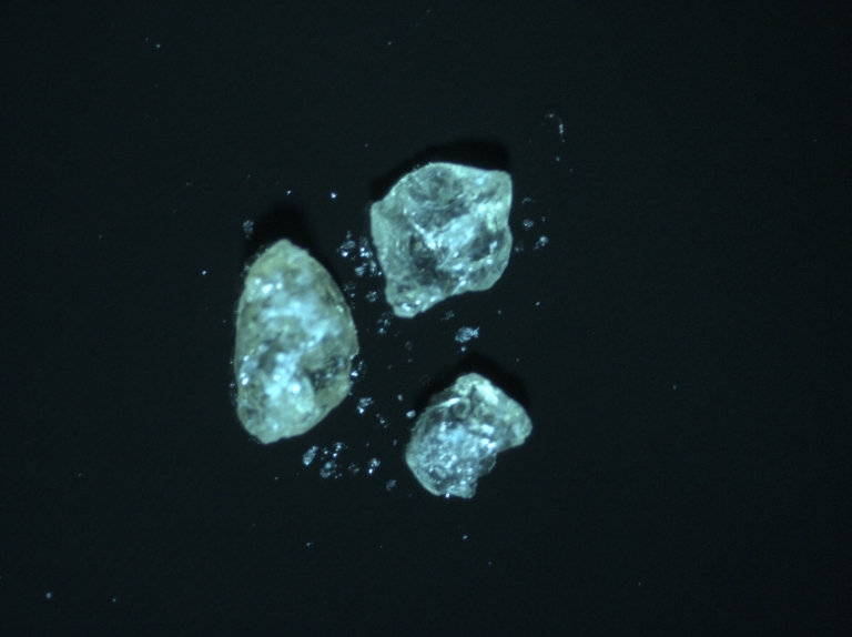
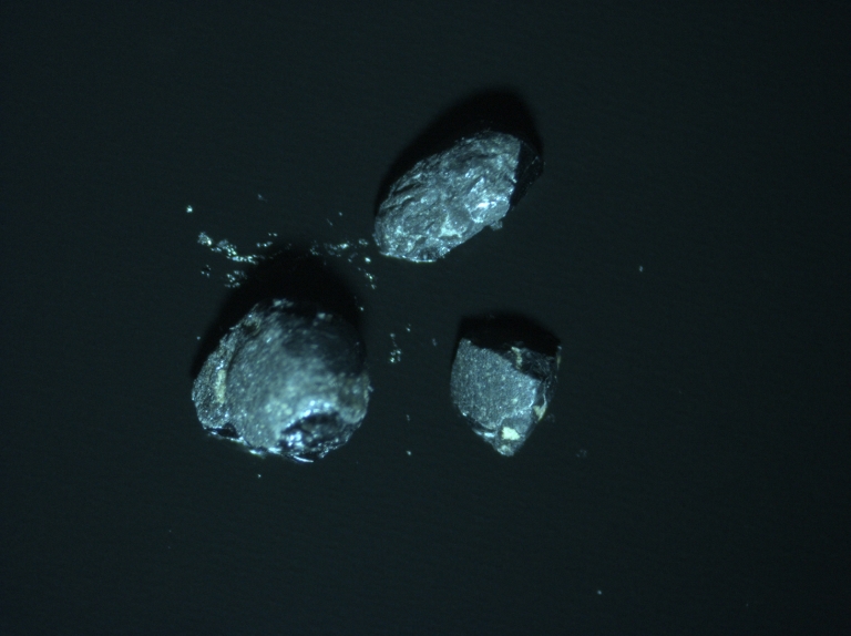
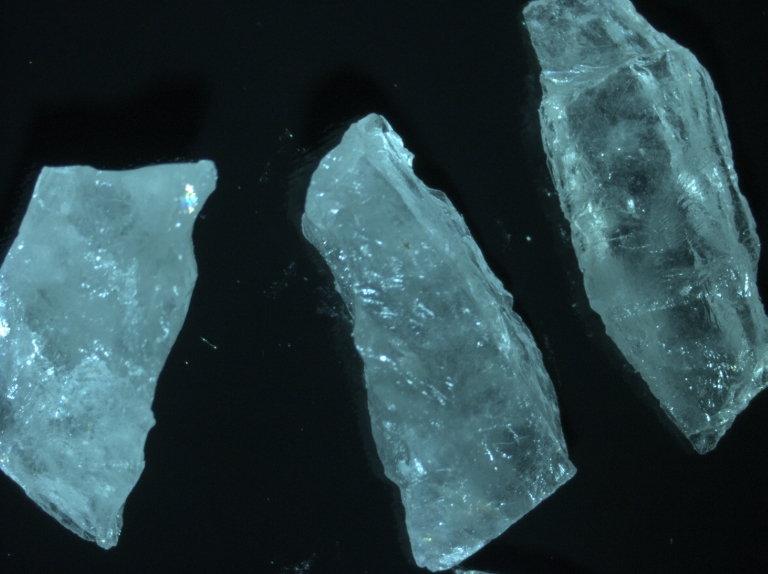
We have five pure minerals. Ilmenite (ILM), Olivine (OL), Pyrope (PYR), Chromite (CHR), and Quartz (QTZ).
Also we have a mix sample that contains all pure sample on it. These minerals are shown as below. (from left to right: 1-ILM 2-OL 3-PYR 4-CHR 5-QTZ)
The mix sample is shown below:
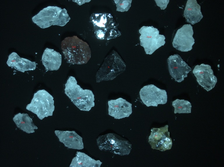
As we can see, the mix sample has all pure minerals that will use in this project.
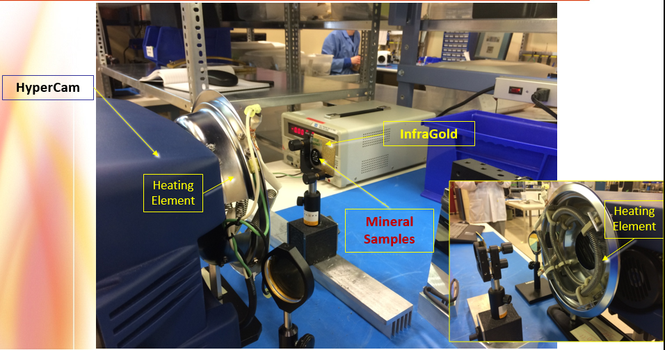
The experimental set-up is shown as below:
The results of pure Pyrope and Olivine by TELOPS camera are shown below:
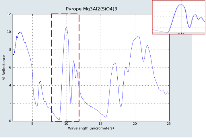
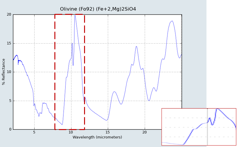
The left one is NASA's result. At the middle is my result. The right one is compare my result and NASA data set.
Our results of pure samples are similar to data set. There is some difference between my results and data set, because my testing condition and
camera and grain size are different from data set.
Also, thr software of Telops (Reveal Viewer) and NASA dataset return us text data. I plot my results with NASA data together.
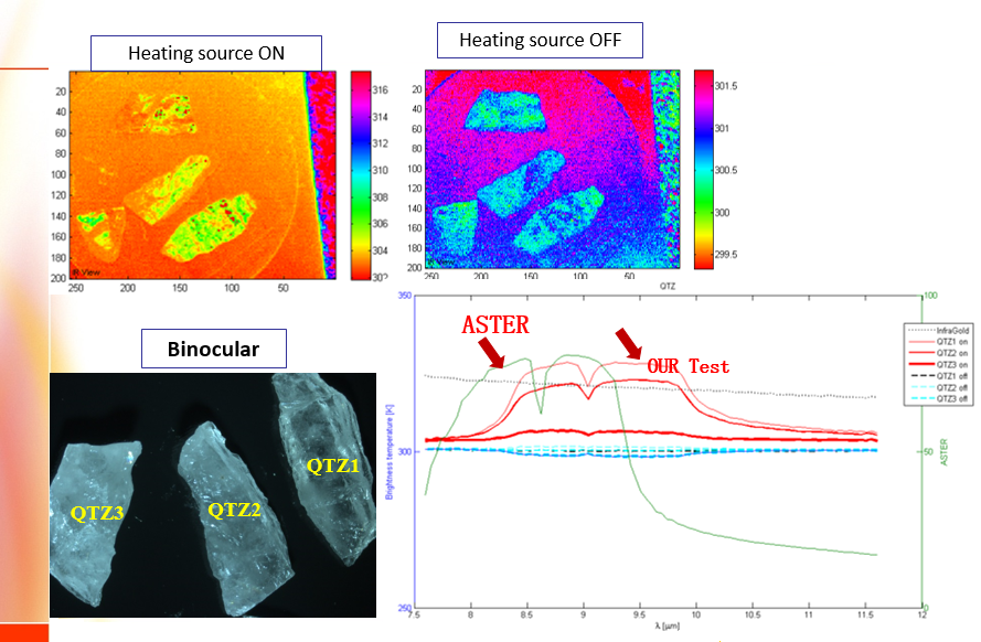
I selected three pixels in three different quartz samples. The test was done in two conditions. First, with heat source on and second, with heat source off.
NASA curve is in source on. As we can see the results, our results is similar to NASA data with small different. Because the sacle of vectors are
not equal and also, both images are took in different spectral bands.
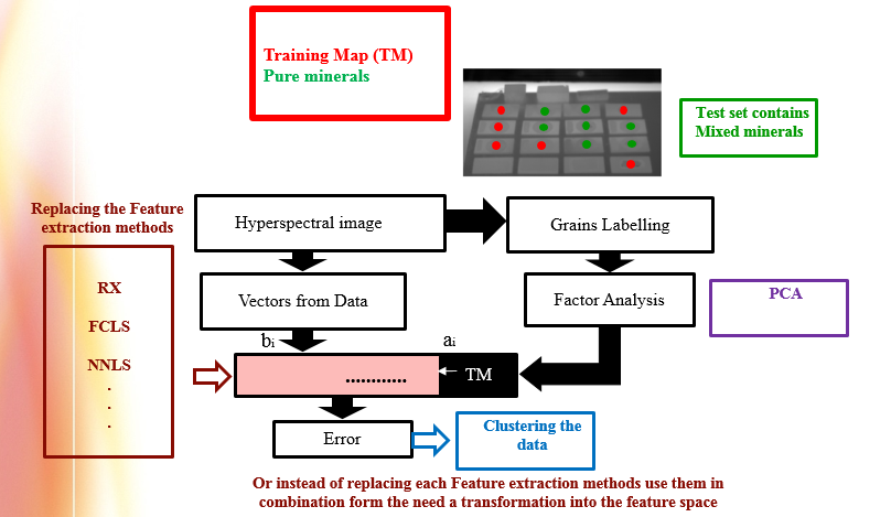
In this project, I took hyperspectral images of pure samples by the Telops Hyper camera. After that, I tray to find samples in mix set.
For doing this purpose, We need classification. First, we use feature extraction techniques to extract pure samples data. for this part I
will use three hyperspectral methods(Spectral Angle Mapper (SAM), Spectral Information Divergence (SID), and Normalize cross-Correlation (NXCC) .
Then, we use machine learning system to find type of samples in mix set. For this part I will use Extreme Learning Machine (ELM)
Here is a sipmle classification example:
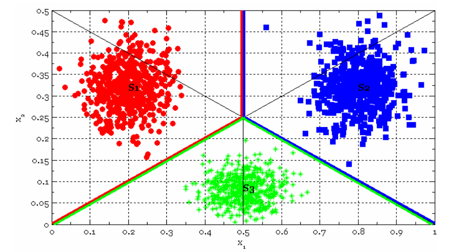
Spectral Angle Mapper (SAM)
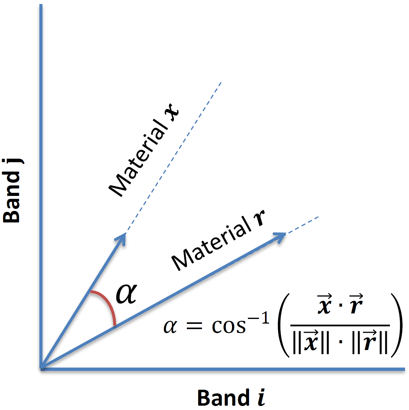
The spectral angle mapper classification (SAM) is an automatic method that compares spectra of image with a known spectra.
Both spectra are as vectors in this method. SAM calculates angle between vectors. SAM algorithm works with vector direction not vector length,
then it is not sensitive to illumination and albedo effects. Finally, we have an image that shows best match at each pixel.
This algorithm works well at homogeneous regions. [5]
In two dimensional, each two point spectrum is a point in band i vs. band j space. The angle α describes the angular separation of two spectra.
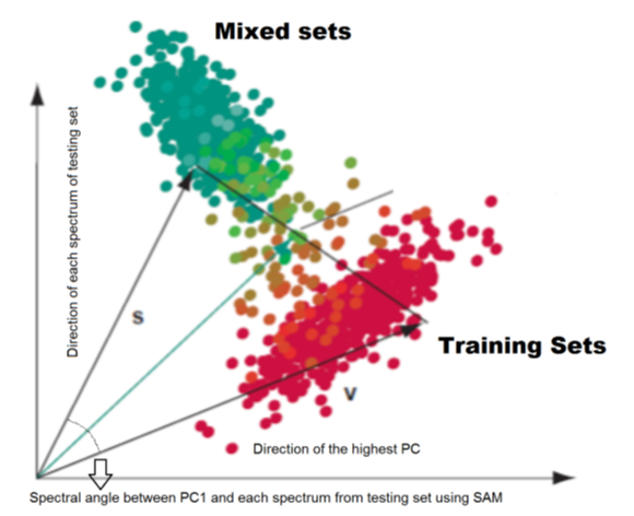
For computing of the SAM, there must be a reference vector as ground for evaluation of the spectral angle difference between
the targeted point and the reference spectra. The common approach for estimation of this angle is related to finding
the endmember spectra from the training set which is modified here through replacing the mentioned reference spectrum with
first principle component attained from the training set. It means first we calculate the principle component analysis for the spectra of
the training set then by finding the representative of the mineral groups, we will proceed with the estimation of the spectral angle
different from the mentioned spectra and targeted pixel spectrum in the testing stage. It is noticeable
that there is not only using the SAM for finding the error difference between the sets,
there will be also spectral information divergence (SID) and Normalized cross-correlation.
Spectral Information Divergence (SID)
Spectral information divergence (SID) is another spectra classification method for hyperspectral images.
This algorithm uses a divergence measure to compare each pixel spectra with reference spectra. If this divergence is small,
the pixel is more likely to reference. Also, we have a threshold for greater divergence.
Some pixels that have divergence greater than this threshold are not classified. [6]
SAM and SID
SAM and SID are both spectral measures. SAM is a deterministic method that looks for an exact pixel match and weights the differences the same.
SID is a probabilistic method that allows for variations in pixel measurements, where probability is measured from zero to a user-defined threshold.
SAM is a physically- based spectral classification that uses an n-dimensional angle to match pixels to reference spectra.
The algorithm determines the spectral similarity between two spectra by calculating the angle between
the spectra and treating them as vectors in a space with dimensionality equal to the number of bands.
SID is a spectral classification method that uses a divergence measure to match pixels to reference spectra. The smaller the divergence,
the more likely the pixels are similar. Pixels with a measurement greater than the specified maximum divergence threshold are not classified.
When you view the SAM and SID classification, you see that the results are similar [6].
Normalize cross-Correlation (NXCC)
In signal processing cross-correlation is a measure of similarity of two functions.
Cross-correlation is similar to convolution. Normalized cross-correlation uses in image processing.
The images can be first normalized. This is typically done at every step by subtracting the mean and dividing by the standard deviation.
That is, the cross-correlation of a template, t(x,y) with a subimage f(x,y) is[7]:
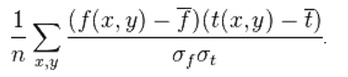
Where n is the number of pixels in t(x,y) and f(x,y) ,f-- is the average of f and σf is standard deviation of f.
In functional analysis terms, this can be thought of as the dot product of two normalized vectors. That is, if:
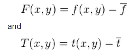
Thus, if f and t are real matrices, their normalized cross-correlation equals the cosine of the angle between the unit vectors F and T,
being thus 1 if and only if F equals T multiplied by a positive scalar.
Hyperspectral images are very big images. They occupied more spaces. For example, one of my results (hyperspectral) is near 3GB.
So, I use PCA to solve this problem and simplicity of procedure.
Principal component analysis (PCA)
Principal component analysis (PCA) is orthogonal lines transformation.
PCA transforms data to new coordinate (smaller) in new coordinate. Greatest variance on the first coordinate (first principle component)
and the second greatest variance on the second coordinate, and so on [7].
Singular value decomposition (SVD) is m×n real or complex matrix.
M = U∑ V*
U is m×m matrix and ∑ is m×n and V* is n×n matrix.
m columns of U are left singular vectors of M. n columns of V are right singular vectors of M.
The left singular vectors of M are eigenvectors of MM*. The right singular vectors of M are eigenvectors of M*M.
The non-zero singular values of ∑ are the square roots of the non-zero eigenvalue of M*M or MM* [7].
Implying the PCA, the reference spectra have attained and applying the mentioned methods for spectral difference provide
the attributes which are given the opportunity for classification process. Here, a single-hidden layer feedforward neural network called
extreme learning machine utilized for the classification of the estimated attributes.
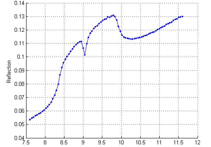
One result of the first PC from a set of the Quartz mineral grain uses as reference of the approaches is shown below:
Extreme Learning Machine (ELM)
Extreme learning machine (ELM) has been proposed for single-hidden layer feed-forward neural networks (SLFNs) for achieve good results
with fast speed. ELM can be extended to radial basis function (RBF). ELM algorithm for RBF is very fast and it produces very good results.
“ELM randomly chooses the input weights and automatically determines the output weights of SLFNs”.
“ELM arbitrary assign the kernels instead of tuning them” [8].
The output function of ELM for generalized SLFNs (take one output node case as an example) is [10]:
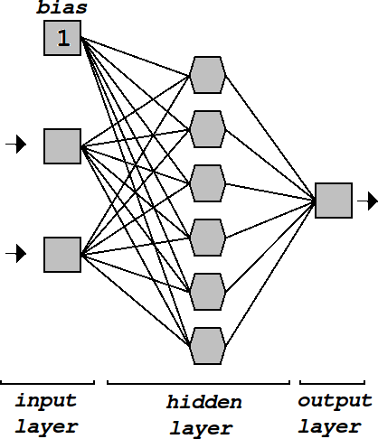
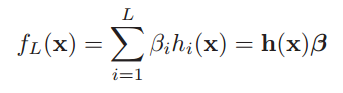
L is number of hidden nodes
Where
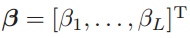
β is the vector of the output weights between the hidden layer of L nodes and the output node, and
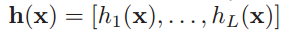
is the output (row) vector of the hidden layer with respect to the input.The function h can be any arbitrary activation function such as: sigmoid, RBF,...
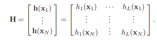
If h activation function is RBF then ELM is RBF too. We can write T = Hβ. T is our target and N×1 vector. H is N×L and β is L×1 matrix.
ELM is to minimize the training error as well as the norm of the output weights
Minimize || Hβ – T||2 and ||β||
Where:
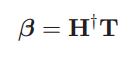
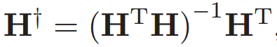
The minimal norm least square method instead of the standard optimization method was used in the original implementation of ELM.
HTHβ = HTt
Least square
Least square has over-fitting effect and this effect is not good. We want to generalization, so we constrain optimization to solve this problem, that leads
to regularization inverse term in the estimation of β as fallow:

Where C is typically determined by cross validation method.
The diagram of my algorithm is shown below. The green point are training sets and the red points are testing set.
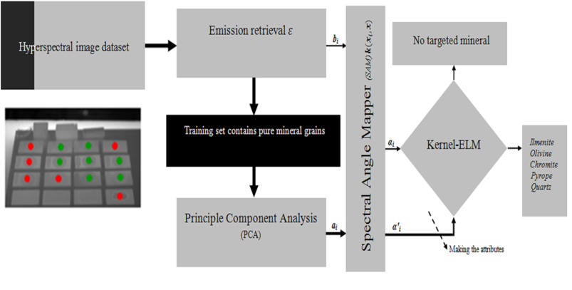
In my algorithm, first I choose the method (SAM, SID, NXCC). Method 1 is HyperSam, Method 2 is HyperSid, and Method 3 is HyperNormXCorr.
Then I defined the name of my samples. I used PCA to calculate the first PC and save it as a mat format. Now I load my data that
I obtained from PCA. I select one of three method and apply method on my data. This is my training part.
The results are saved in text format (see ‘code/elm_kernel/ 1vsAll’). First column of text contains type of mineral.
We have five different minerals, so we should create five training text. Each text has five parts
(the rows divide to five part and each part contains information of training, like angle in SAM), where first column is one we have
that mineral because I used binary classification. Where first column is zero we do not have that mineral.
For example if the second part of first column is zero we do not have second mineral in this training.
First training text, trains on first mineral that I defined before. I manually select the region of minerals in mix sample.
I knew the position of samples in mix set, then I manually select them and saved data in excel file (see ‘code/mineral_test.xlsx’).
Because I want to test accuracy of my algorithm. Now, I apply training results to this regions. For example,
I know the position of Quartz in mix sample, but my machine does not know that. I apply the training result of quartz to position of quartz
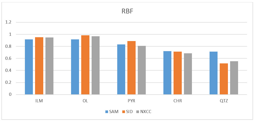
in mix set. The results of testing are saved as text (same as training). In ELM I used RBF kernel.
Finally, I gave result of training and testing to ELM kernel (kernel2) and ELM returned me the testing accuracy.
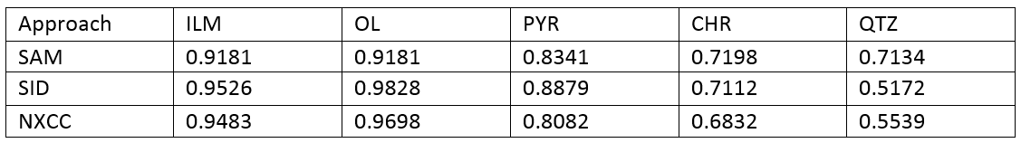
The result of testing accuracy are shown below:
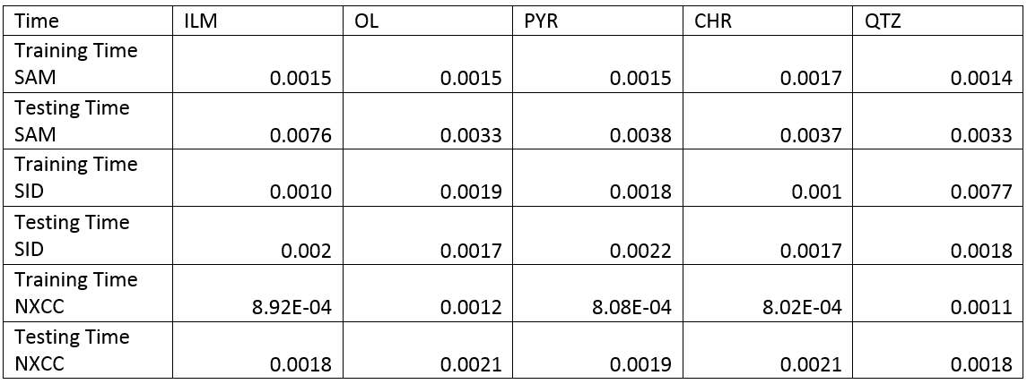
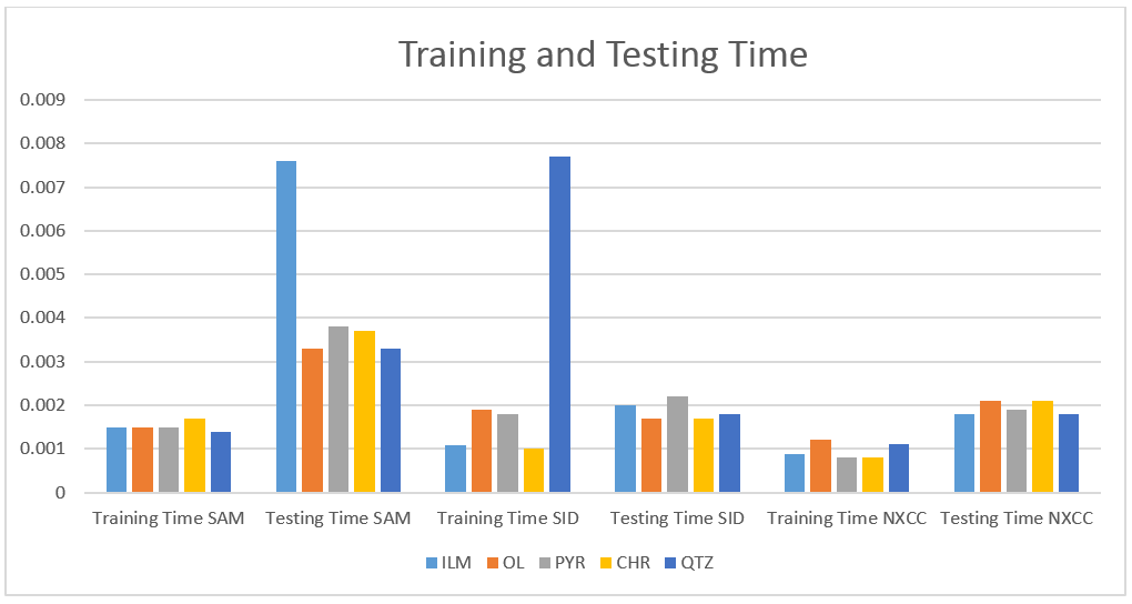
Also, training time and testing time are shown below:
Discussion
As we can see in the results of testing accuracy these three methods are almost similar and have same results with little difference.
For ILM and OL SID and NXCC have same results and their results are better than SAM. SID has best results for PYR.
For CHR SAM has best result. This result is almost the same as SID results but both are better than NXCC.
For QTZ SAM has best result. SID has bad result for QTZ.
For the training and testing time NXCC has best results. The NXCC is very fast hyperspectral method.
SAM is not very fast in compare with two other methods. For testing ILM by SAM method we will have long time to test this sample.
Also, we have this problem in training quartz by SID method.
The proposed study has shown the application of the hyperspectral Infrared in the (7.6-11.6 µm) for identification of mineral grains
through PCA based SAM, SID, NXCC and supervised learning classification. Infrared imaging and hyperspectral techniques have been used for
identification of the minerals in the satellite imageries and quality control. The images are in the long wave infrared, and provided promising
results for some mineral grains such as Quartz and Olivine in comparison to other mineral grains such as Ilmenite, Chromite and Pyrope in this
infrared wavelength. However, the signature of Olivine and Ilmenite was not strong, similar to that of Quartz grains.
The results of the classification indicate considerable recognition outcome for identifying the mineral grains.
Generally the SAM has more sensitivity for the shifting factor in the spectrum as compare with SID and NXCC.
It depicts in Quartz mineral grains case because of the very good similarity between the reference and the targeted points
(it is more due to high visibility of the signature of Quartz in the 7.6-11.6 µm). In the case of ilmenite, as there is no
signature regarding the spectrum there will be an only similarity in terms of the angle different between the target and reference.
There are some reasons for this problem which are the poor resolution of FIRST image acquisition or the size of the grains,
as well as the similarity and weakness of the mineral signatures. Furthermore,
there are many other parameters in radiometry which may affect the accuracy, such as the non-uniform surface of the grains.
Conclusion
The presented approaches SAM, SID, and NXCC, which are normally used for applications in satellite imageries.
These methods were applied to the identification of mineral grains in a laboratory environmental situation.
Applying SAM, SID, and NXCC involve the use of the endmember which is considered as a reference for finding the spectral angle.
Here, PCA based methods solved this difficulty by finding the principle component calculated from the training set and used this for
the extraction of the features. A kernel ELM classified the mineral grains in a supervised way. The classification was conducted in the
binary classification scenarios. The results indicated promising accuracy for the proposed approaches.
Moreover, there some missing signatures in the spectrums led to some miss-classifications. In future work,
the low resolution lens of the spectrometer or small size of the mineral grains and their non-uniform surface need further attention.
Future works
For future works we can use other hyperspectral techniques such as: Reed-Xiaoli Detector (RX), Fully-constrained least squares (FCLS),
and Non negative least squares (NNLS).