Project #5 : High Dynamic Range
Submitted by: Razieh Toony
April, 2014
Project Overview :
Human see the world with range of intensity and color. The dynamic range of radiance, generally speaking, is from 1 to 1000, or even larger. However, as the images are often stored in 8-bit format, the maximum intensity that can be saved is 255. Sice some large/small radiance values are cropped, even the modern camera are unable to capture the full dynamic range of encountered real-world scenes.
With a singel image, there may be areas in a photograph that are too bright (overexposed) or too dark (underexposed). The concept of HDR is to display an image by combining the whole range of data from multiple exposures. Actually, we can create an image in which has better details in all spots while it is impossible with one exposure.
This algorithm can be split into two parts
1) The method first recovers the radiance map of the scene, using the approach outlined in "Recovering High Dynamic Range Radiance Maps from Photographs, P. Debevec, J. Malik, SIGGRAPH 1997"[ [1] ]
2) Then, the method uses a local ton mapping algorithm ("Fast Bilateral Filtering for the Display of High Dynamic Range Images, F. Durand, J. Dorsey, SIGGRAPH 2002") [ [2] ] to display the resulting radiance map.
Part 1 : High Dynamic Range Imaging
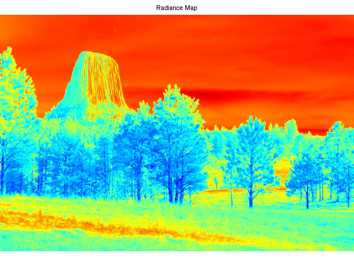
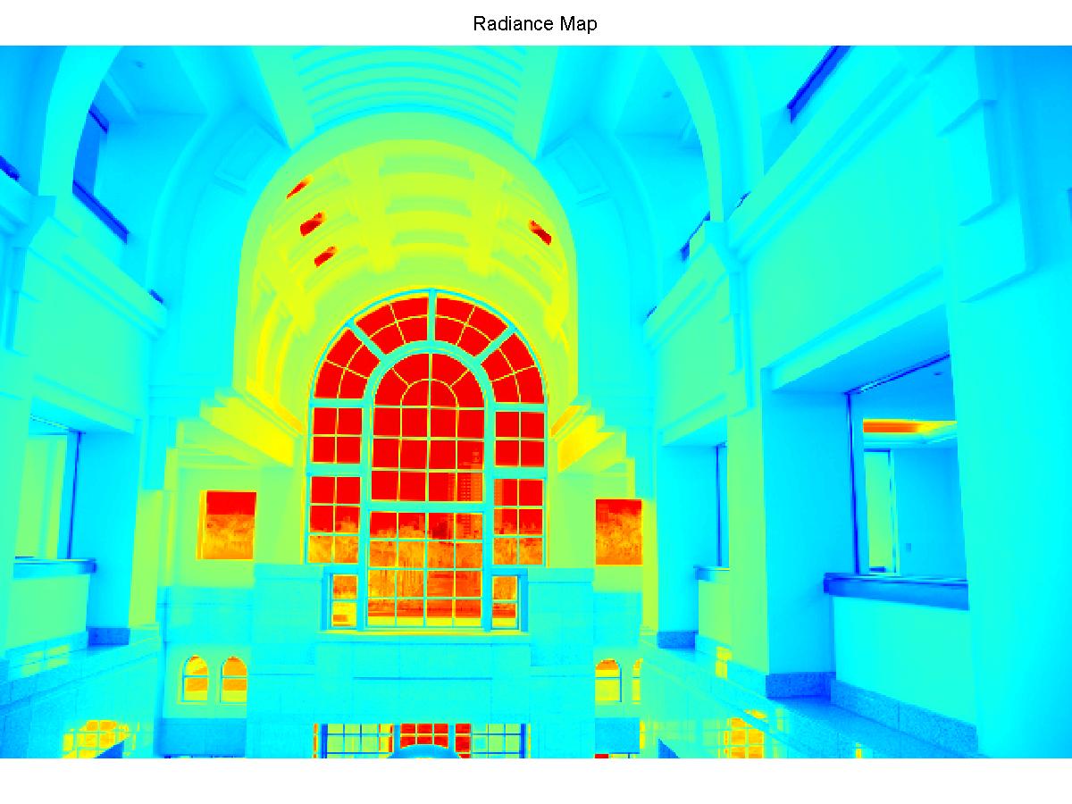
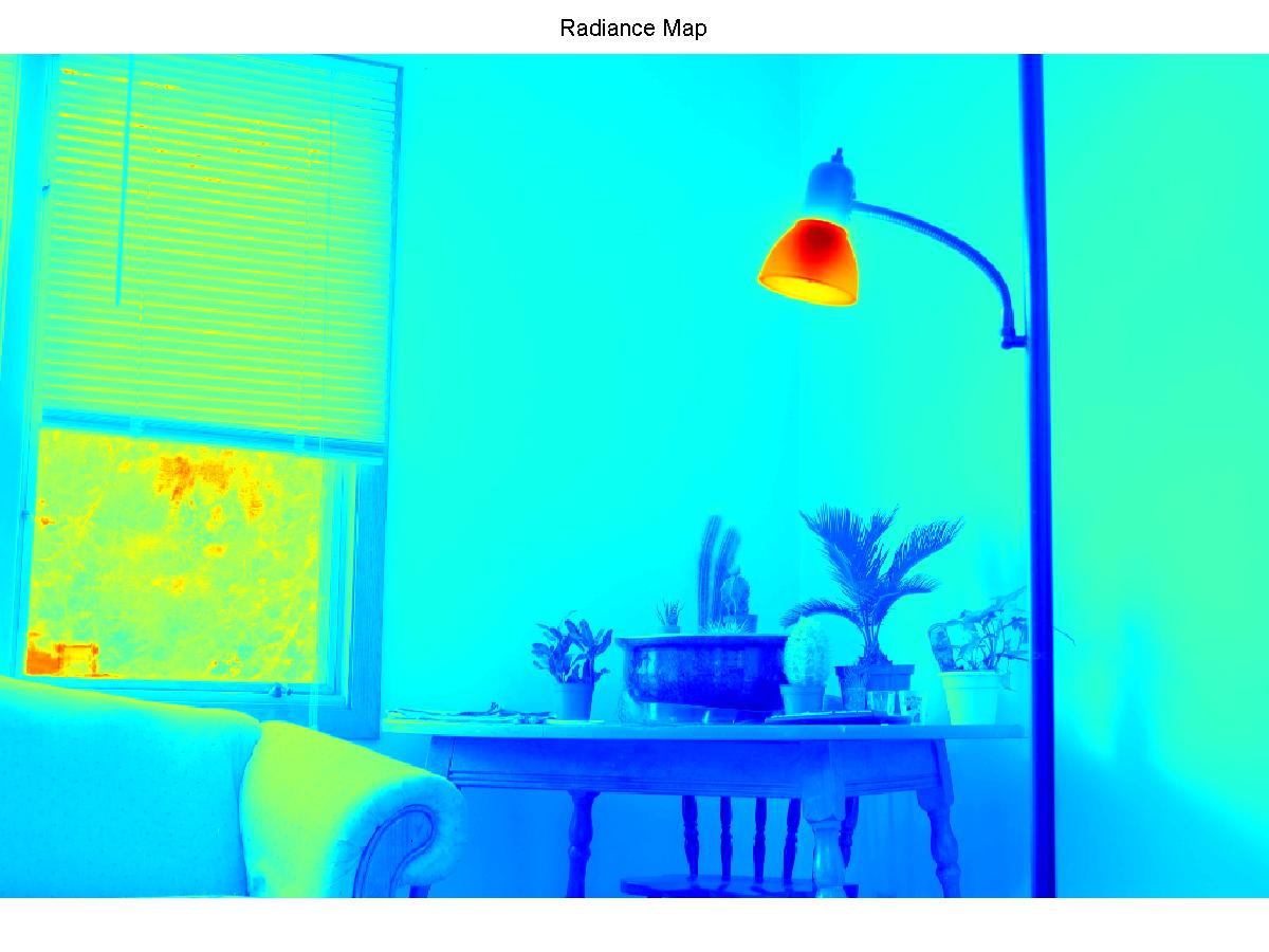
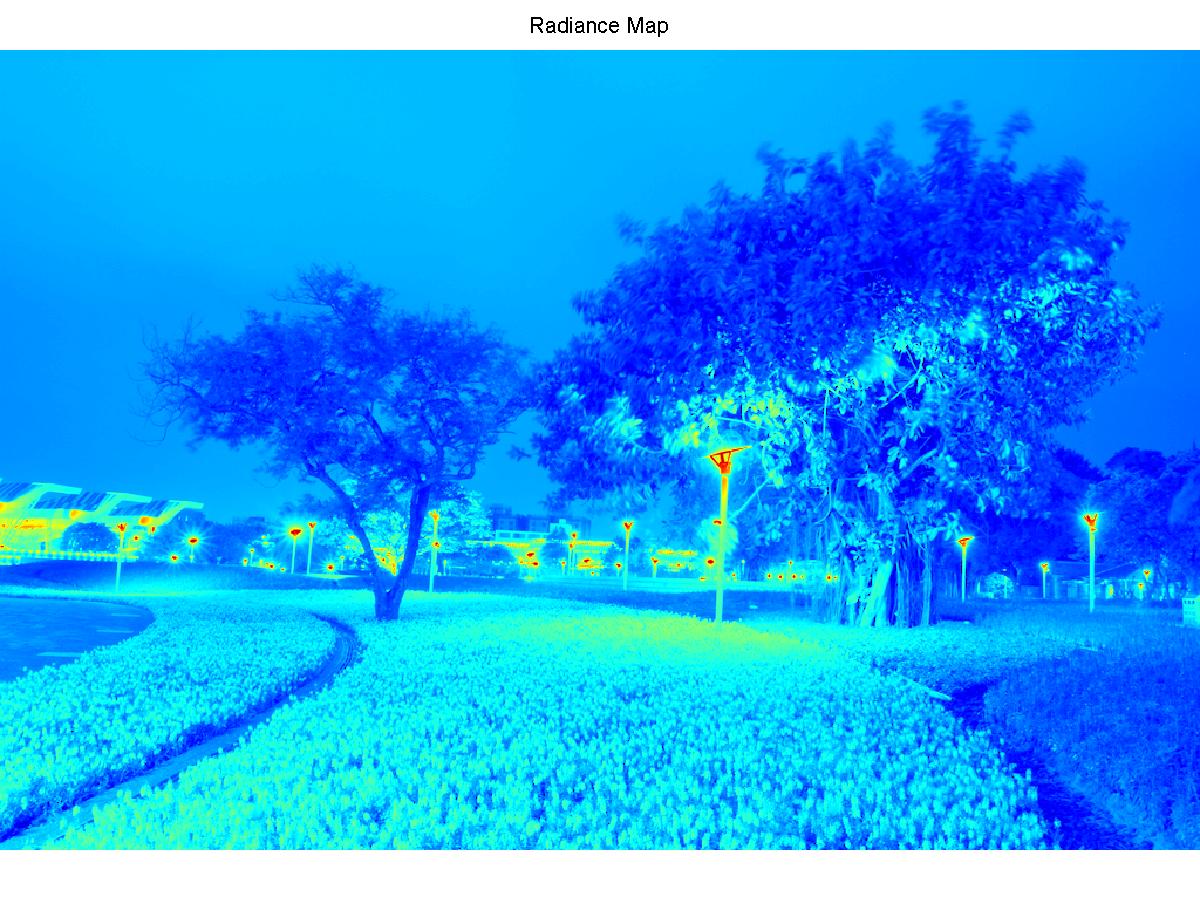
A radiance map is an image that represent the true illuminance values of scene. Radiance map reconstruction consists two main step :
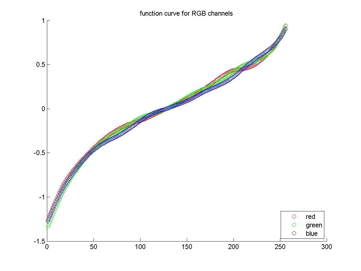
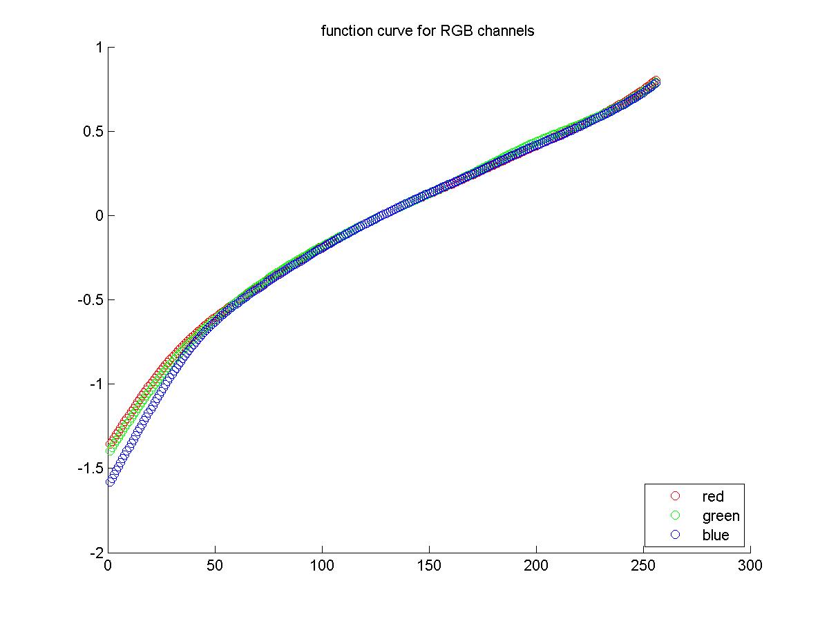
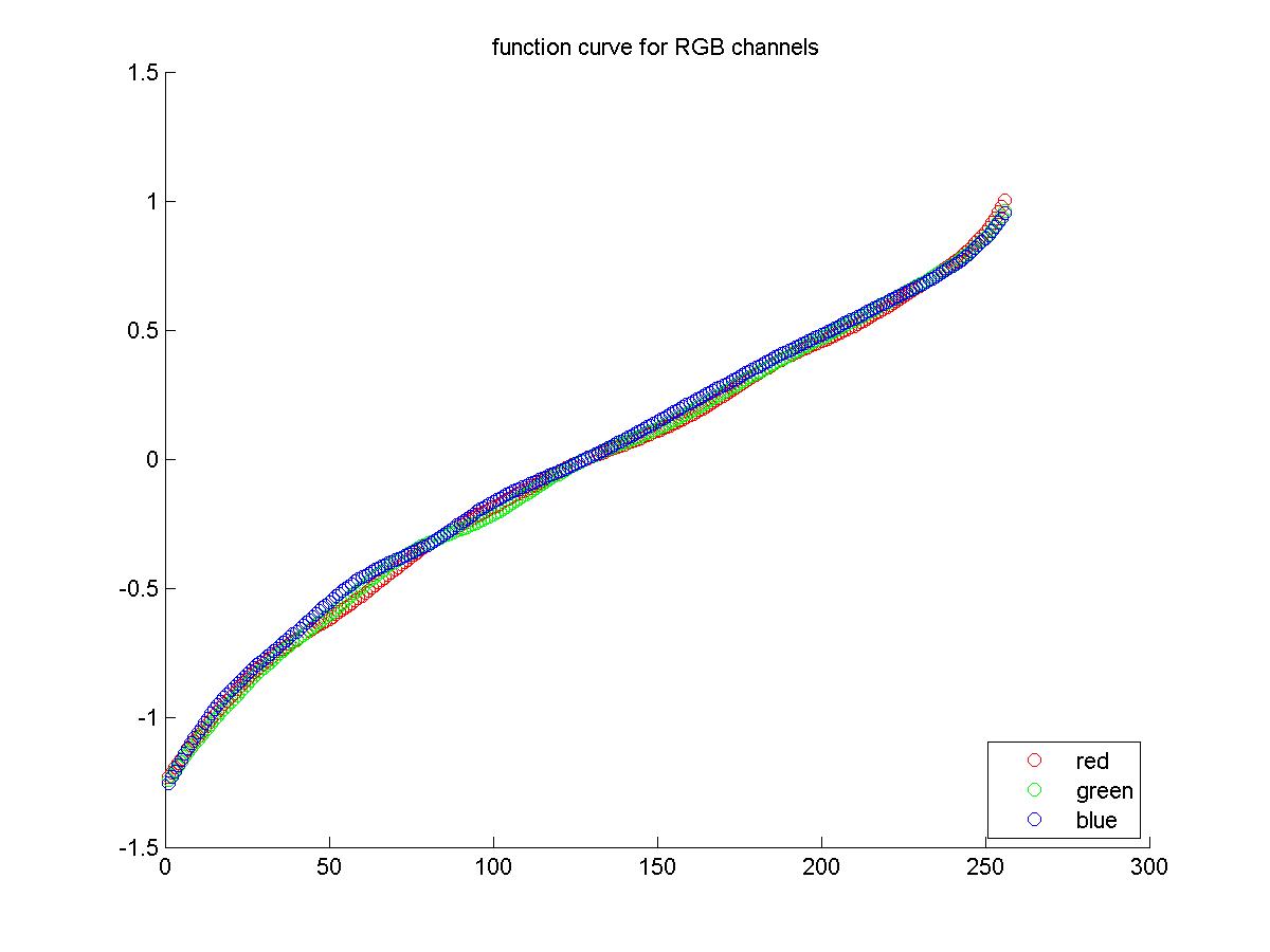
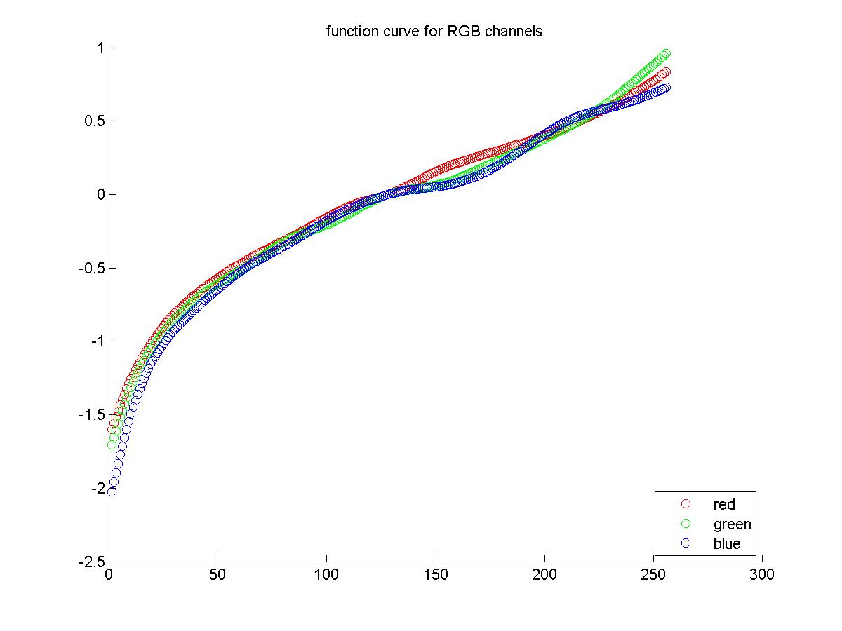
1) Recovering the responce curve between pixels and real radiance
2) Mapping the observed pixel values and exposure times to radiance
It is assumed that images are taken of the same scene with different exposure.With these images, I randomly sample many positions and get the corresponding pixel value in each image. Each pixel value is a function of the exposure time multiplied by the radiance value. In order to find the radiances of each of these pixels, we need to find the function that maps that relationship of pixel value to exposure time: Zij = f ( Ei * Δtj).The value Zij is the pixel value for pixel i in image j and it is a function of scene radiance Ei and exposure time Δt.
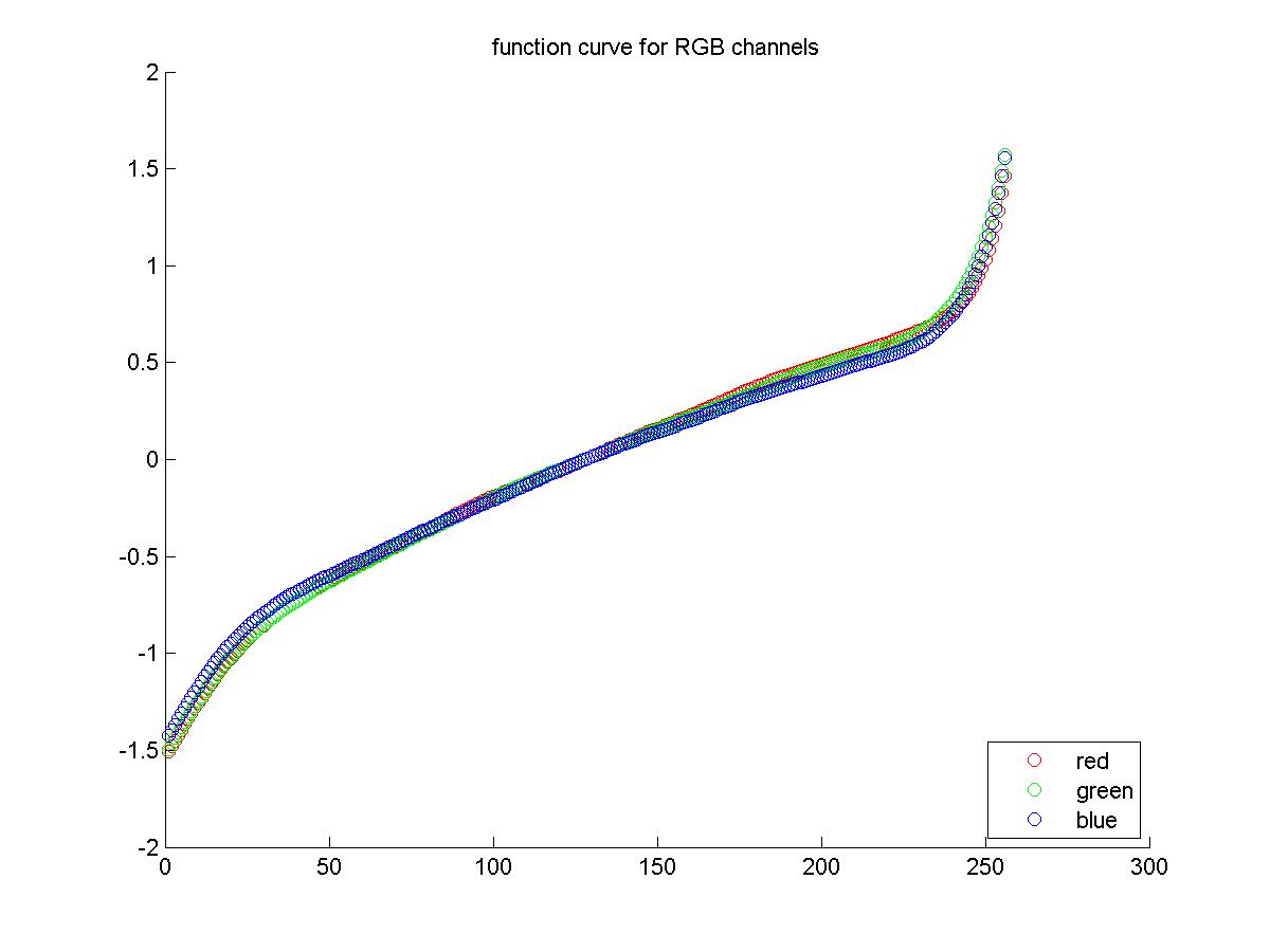
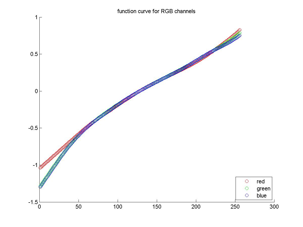
Because this function could be a fairly complicated response curve, it's easier to solve for function g which is : log of f's inverse. Therefore, g maps pixel values to the log of exposure values : ln( f-1 ( Zij ) ) = ln( Ei) + ln( Δtj), given that g = ln( f-1 ). Then we can sum up that : g(Zij) = ln(Ei) + ln(tj)
As I have sampled many different positions, I can build n equations where n is the number of samples. This is still not enough for solving the equation. I suppose the response curve is a smooth and monotonic curve, since a larger radiance won't correspond to a smaller pixel value. Then I give the smooth part a lambda value, which is used to adjust the weight of the smooth part and I also give different weights for different g. This weighting gives less weight to pixels that may be either over or under-exposed. The last thing we add is the equations force the second derivative of g at all points to be roughly 0. Finally, we have an over-constrained linear system of equations which MATLAB can easily solve bu using singular value decomposition (SVD) method(x = A\b)
The second step is to build the radiance map. Because I have got all the possible g from the last step, the radiance map is easily obtained by simple substitution. I reuse the weighting function to give higher weight to exposures in which the pixel's value is closer to the middle of the curve.
Part 2: Tone Mapping
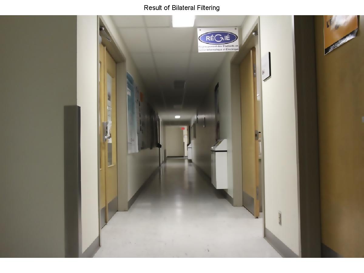
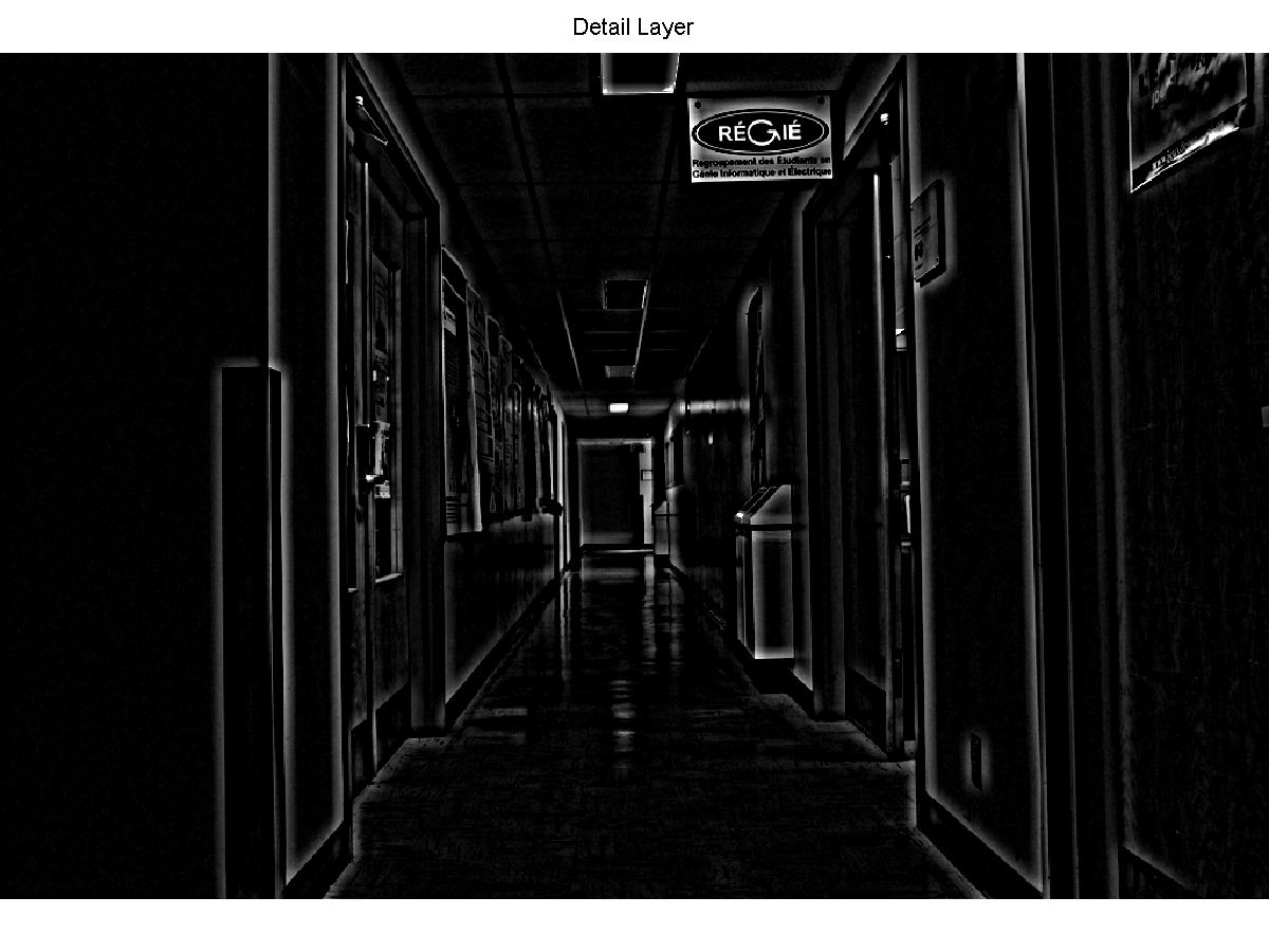
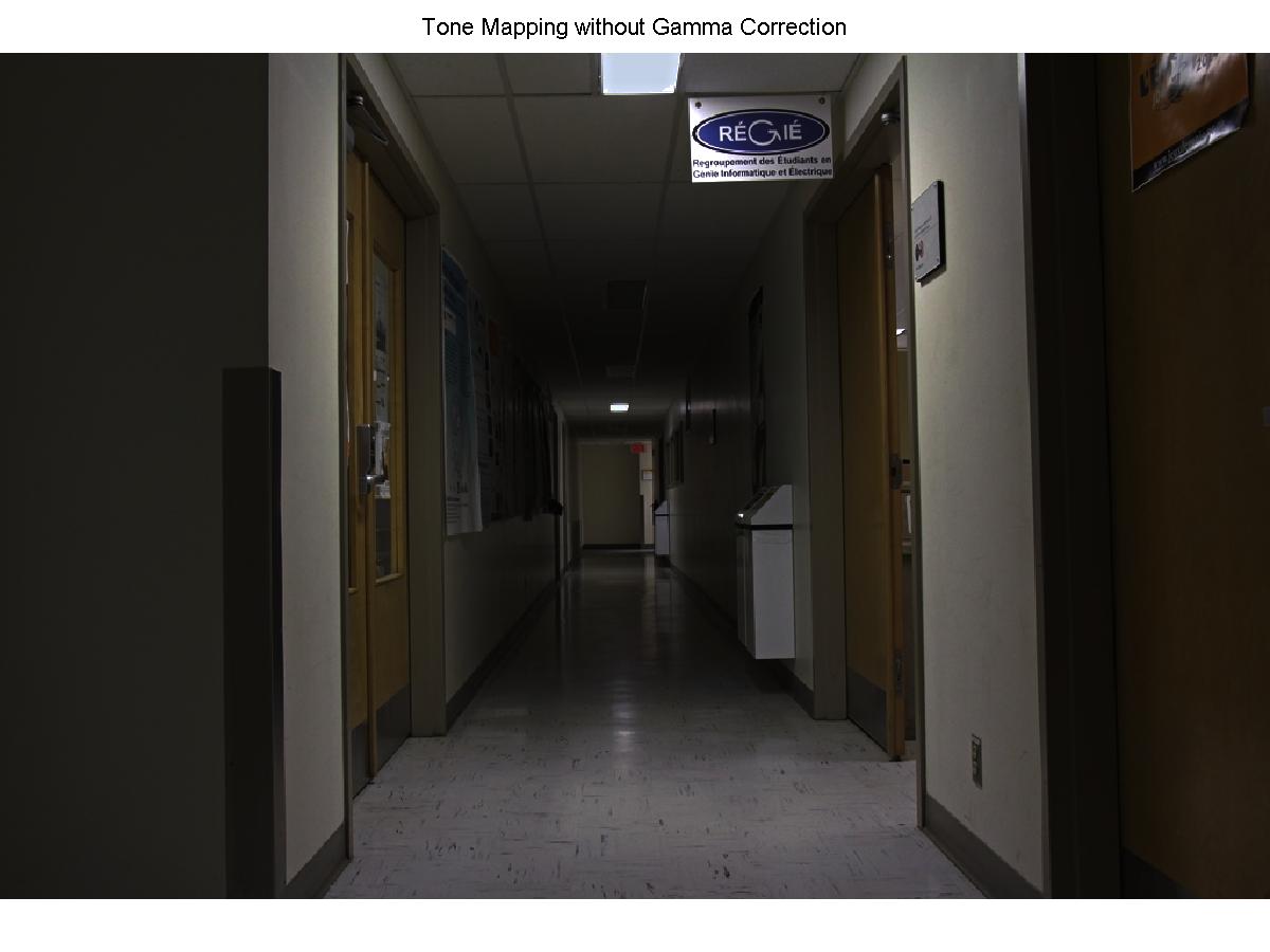
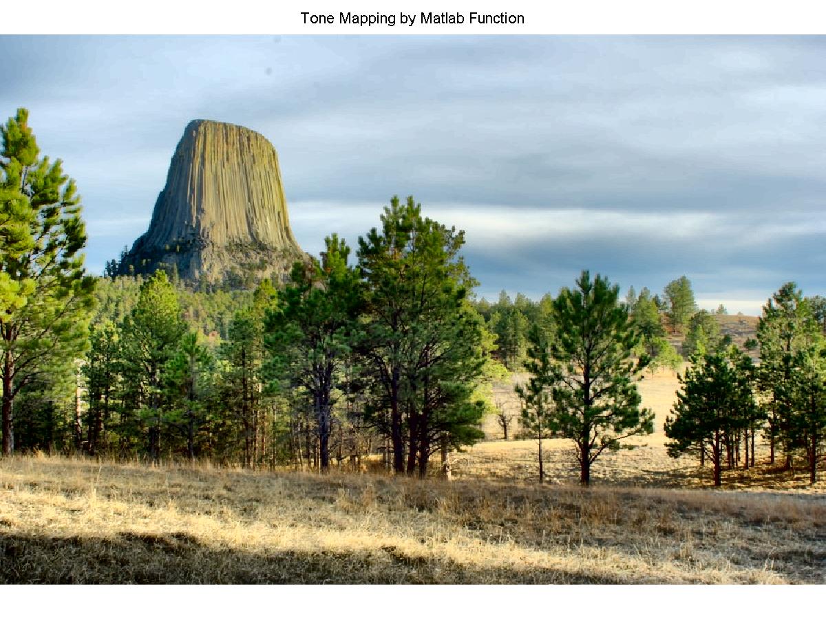
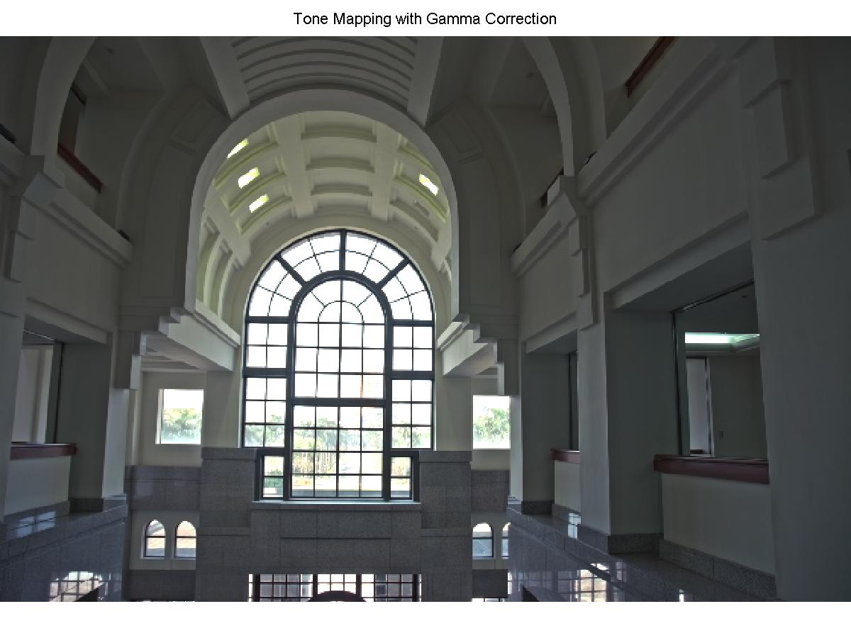
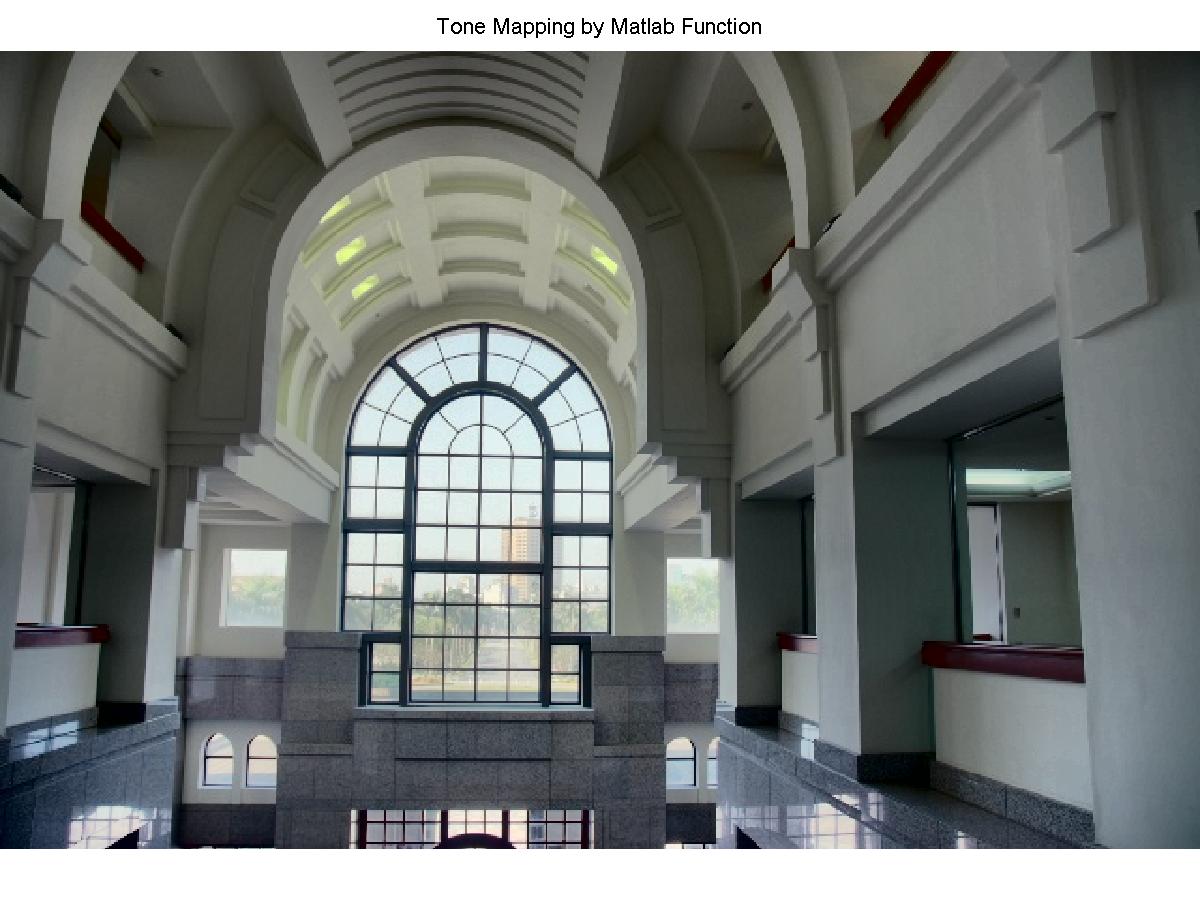
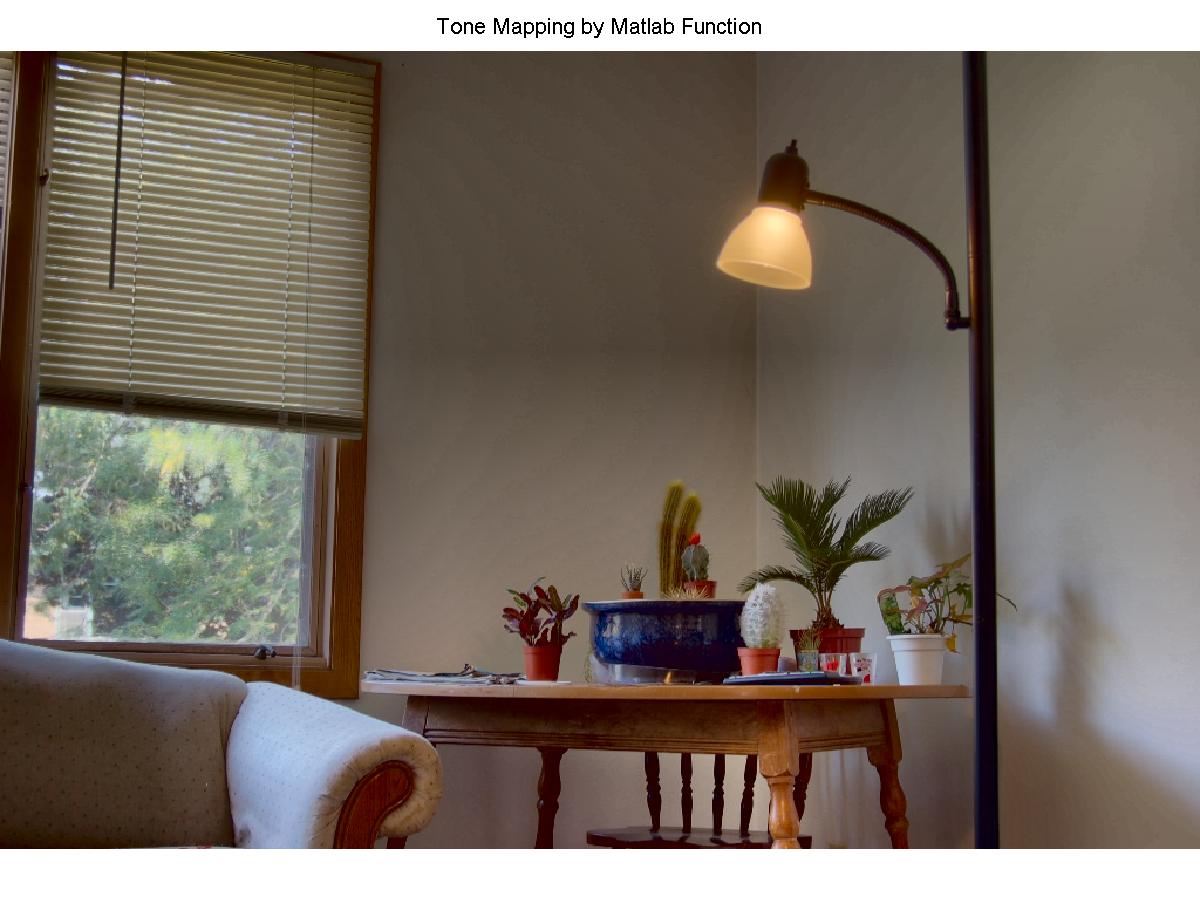
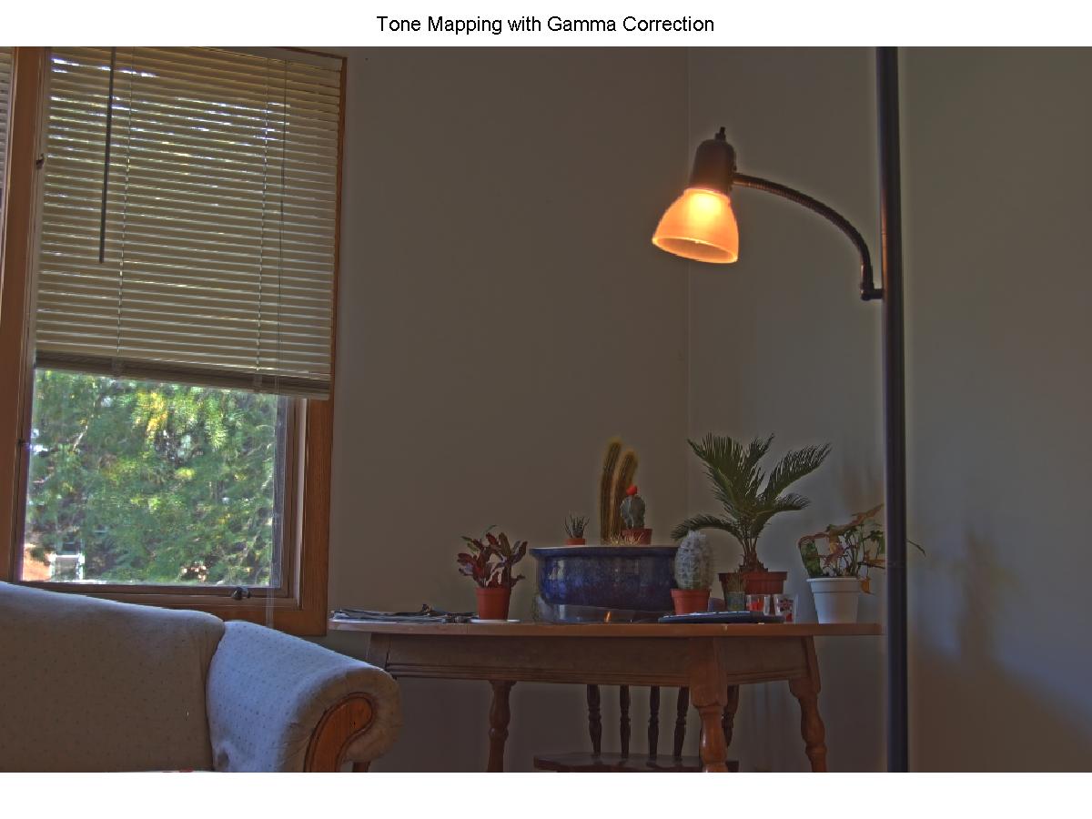
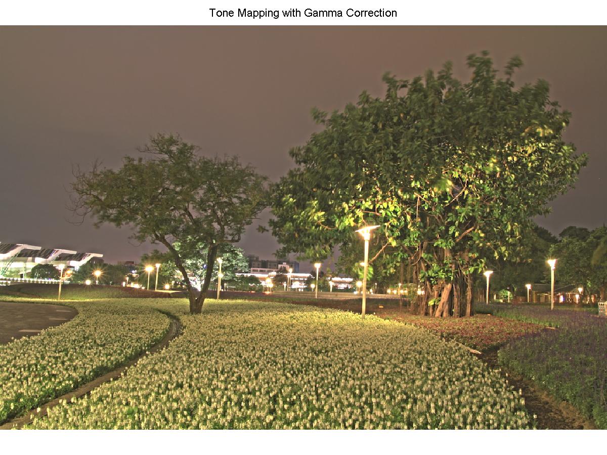
Converting HDR to a displayable image on normal displays is called tone mapping. Tone mapping operators can be classi?ed into global and local techniques. Global techniques use the same mapping function for all pixels. In contrast, local operators use a mapping that varies spatially depending on the neighborhood of a pixel. Most local tone-mapping techniques use a decomposition of the image into different layers or scales. Once the radiance map was recovered, we like to map the world radiance values to a small range which is suitable for visualization. This procedure makes use of what is called bilateral filtering. Bilateral filtering is a method of blurring an image that only blurs similar parts of the image but maintains as many of the edges as possible. To locally tone map the image, we use a biltaeral filter on the intensity of the image, and then extract the details by subtracting the blurred image from the original. We then scale the blurred version to have a more even contrast. Lastly we add the detail and color back into the image. The result is followed by a gamma correction. Indeed, Gamma compression makes the image brighter. Different images may need different gamma value.
In short:
1) Compute the intensity (I) using a luminance function.(I = 0.2126 R + 0.7152 G + 0.0722 B Source:Wikipedia)
2) Find the log intensity, L, of the input radiance map
3) Seperate L into a base layer, B, and a detail layer D, using a bilateral filter
(The bilateral filter returns the base layer, B so that the detail layer can be computed using D = L - B )
4) Scale the base layer
5) Combine the base and detail layers and restore color channels
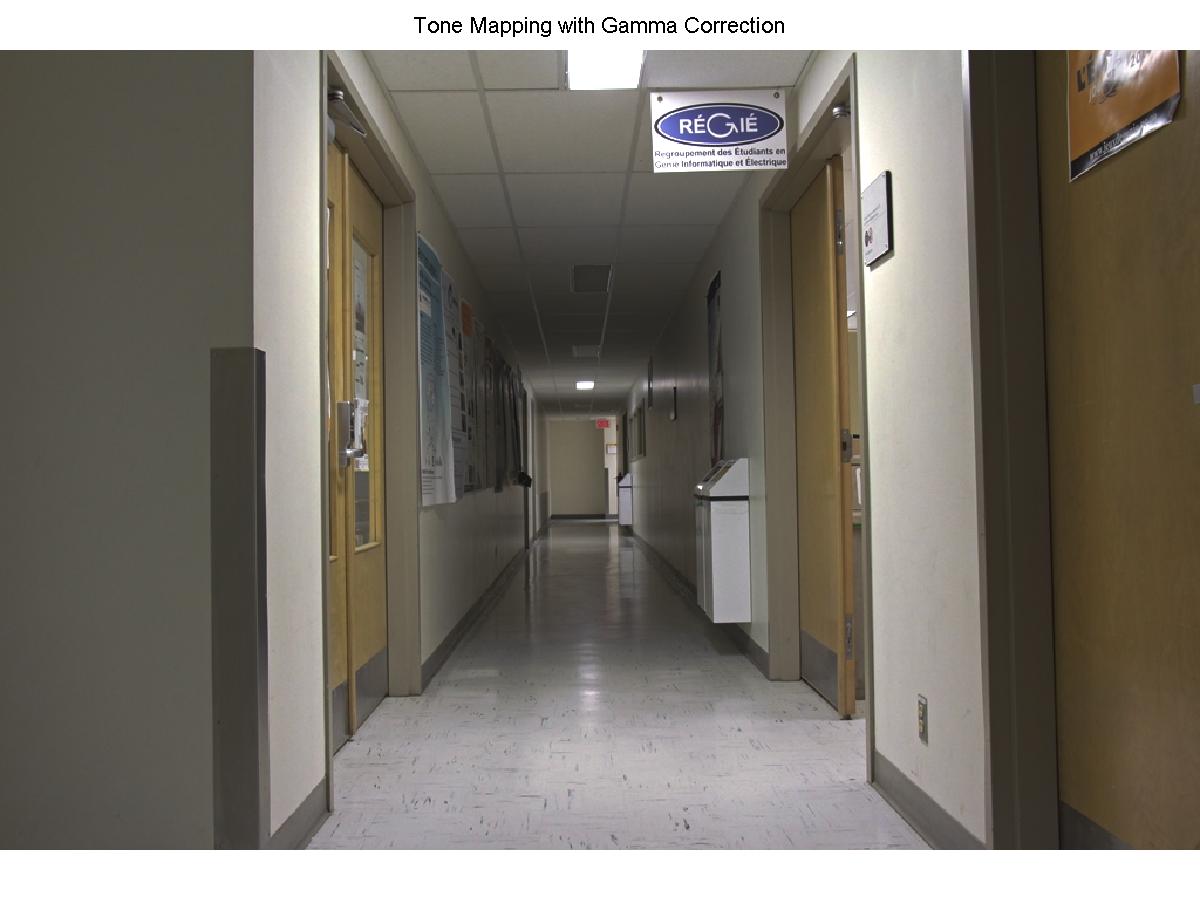
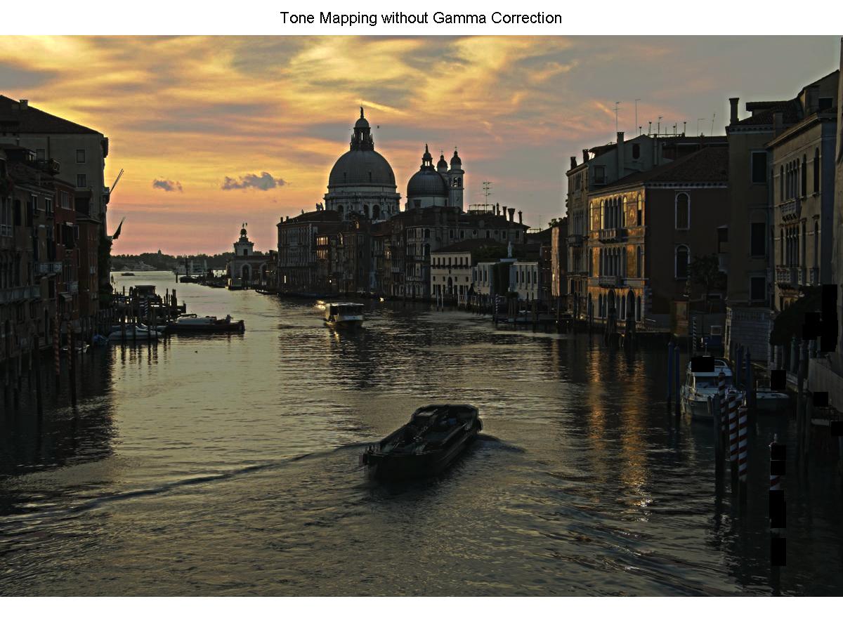
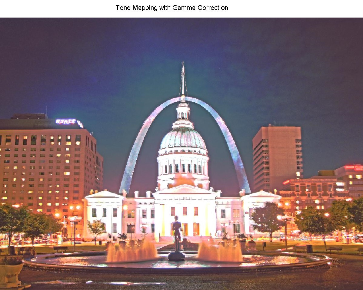
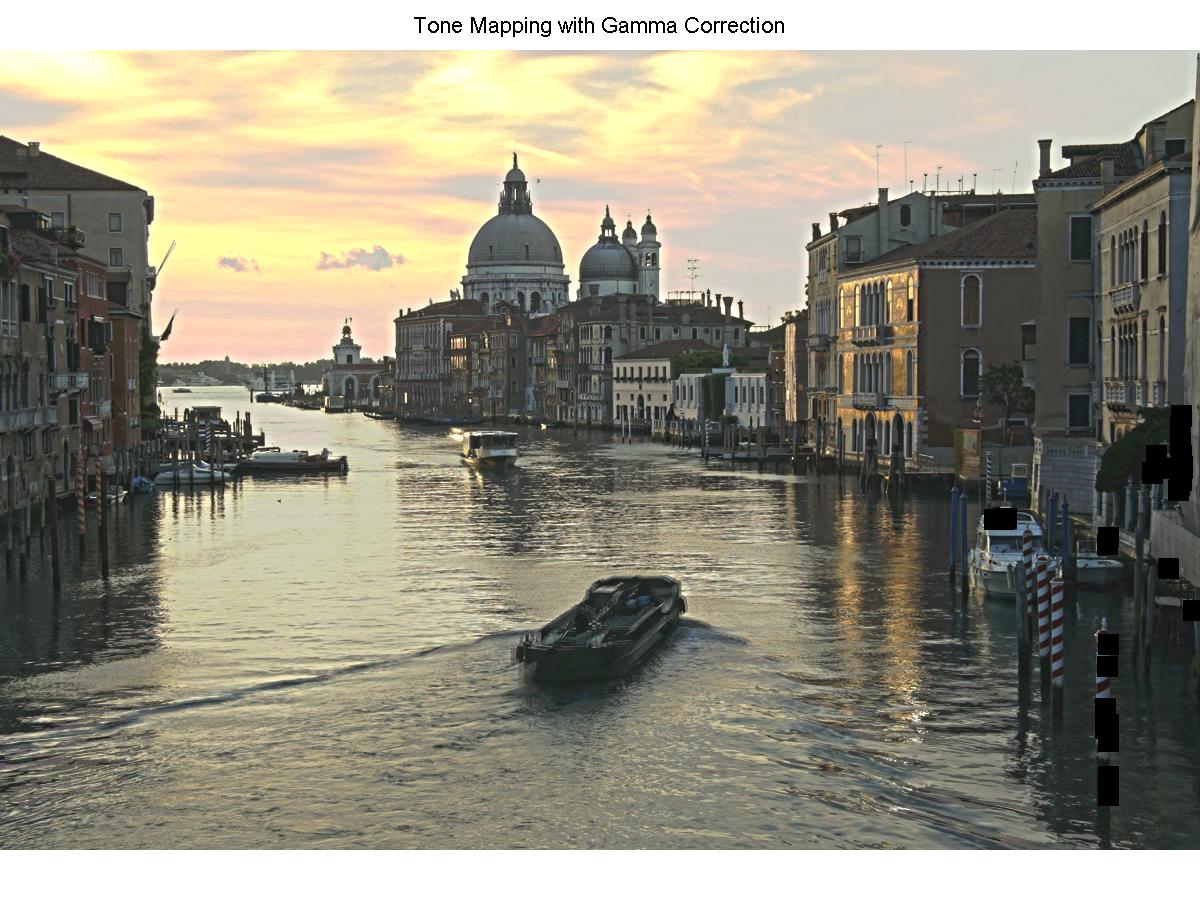
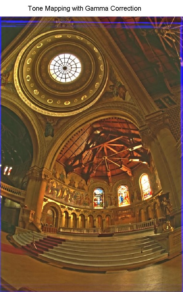
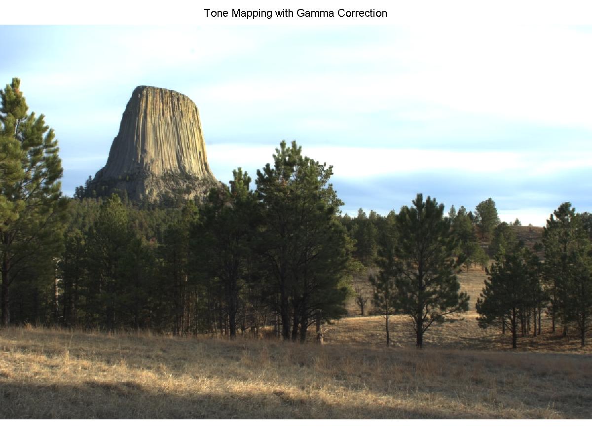
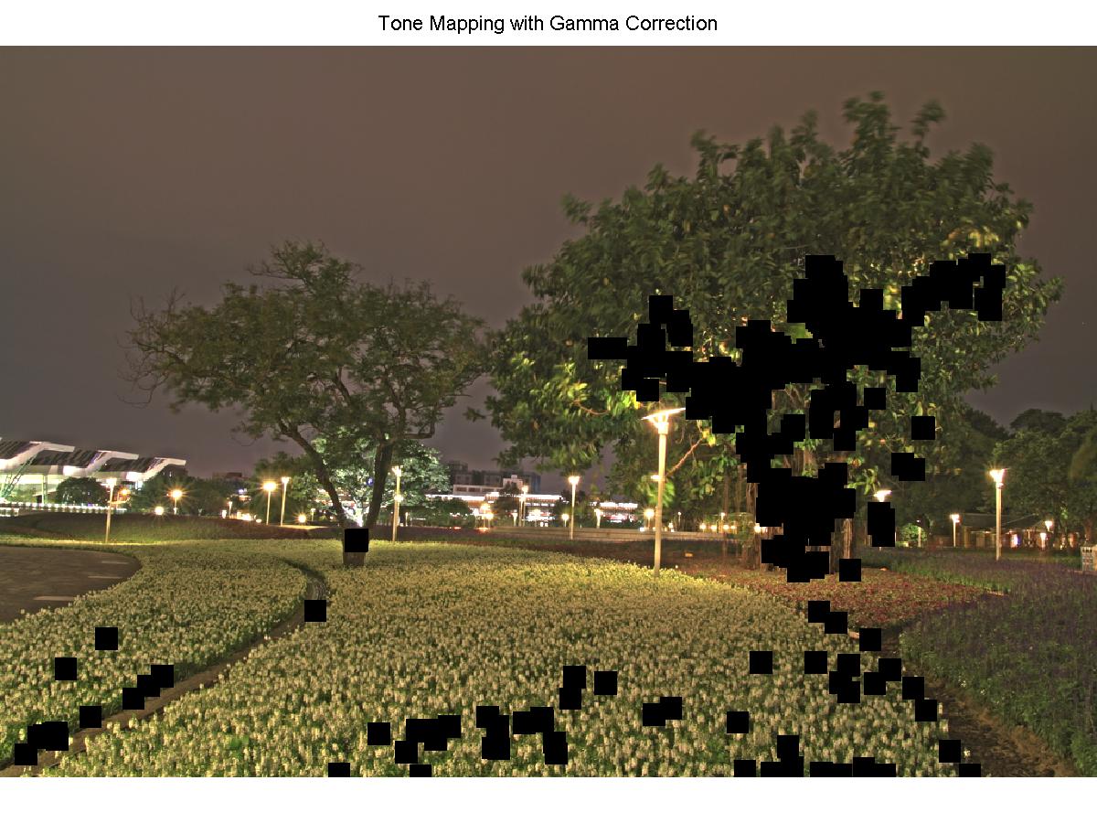
6) Gamma compression (In bellow you can see the effect of Gamma correction)
3) Result
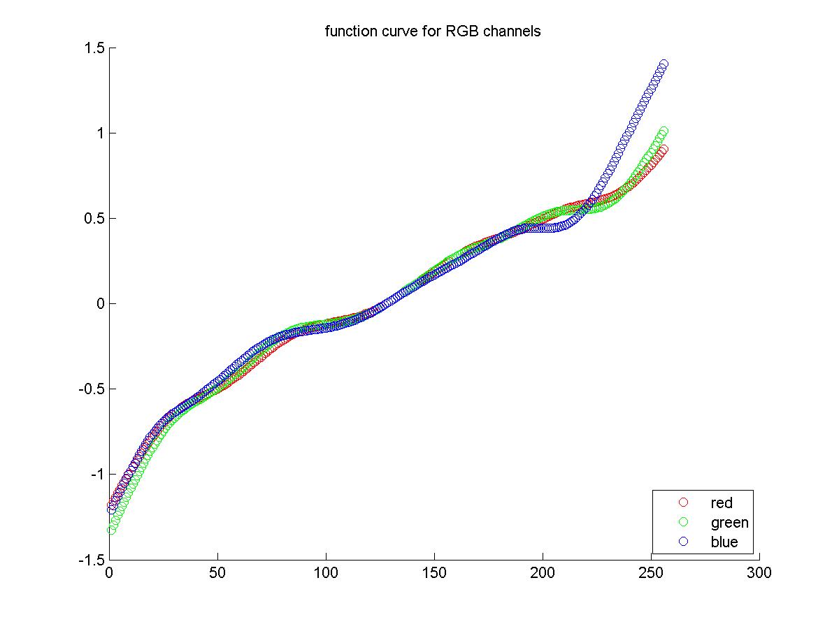
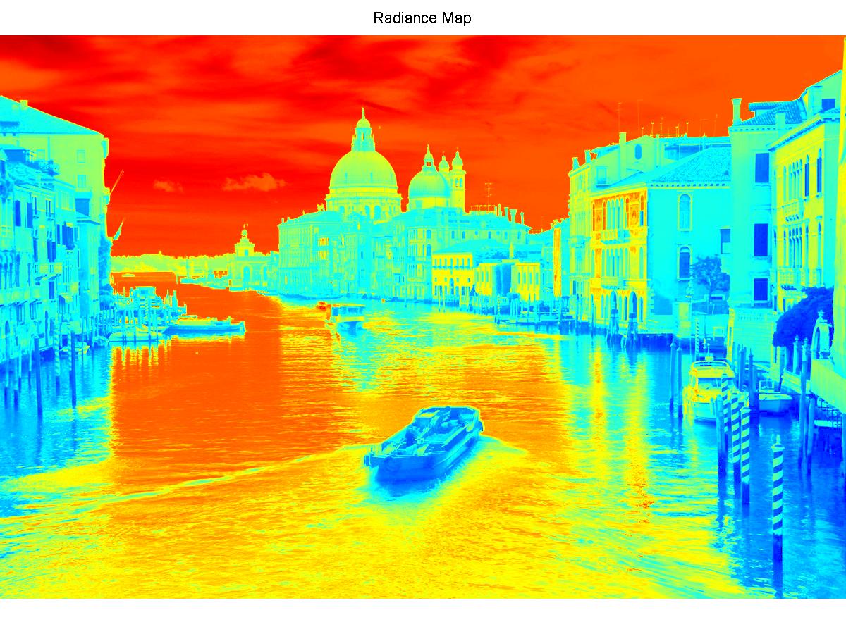
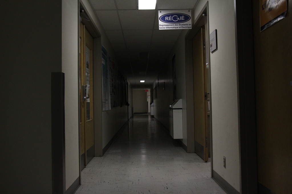
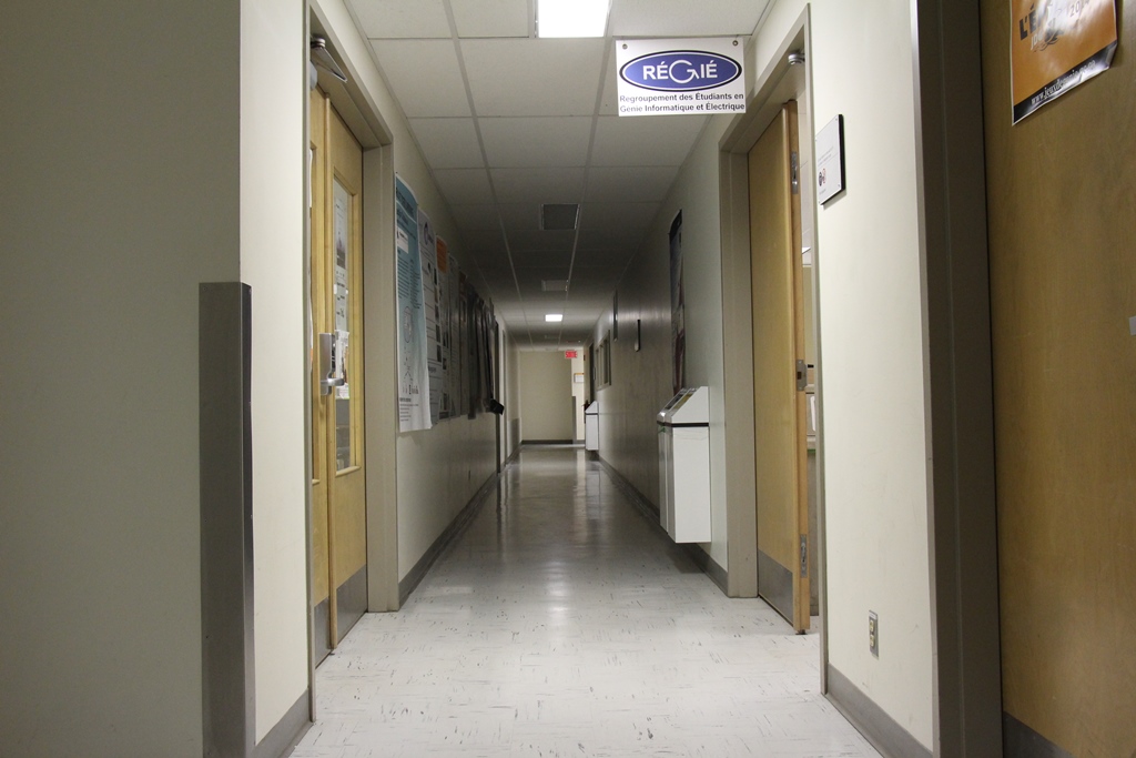
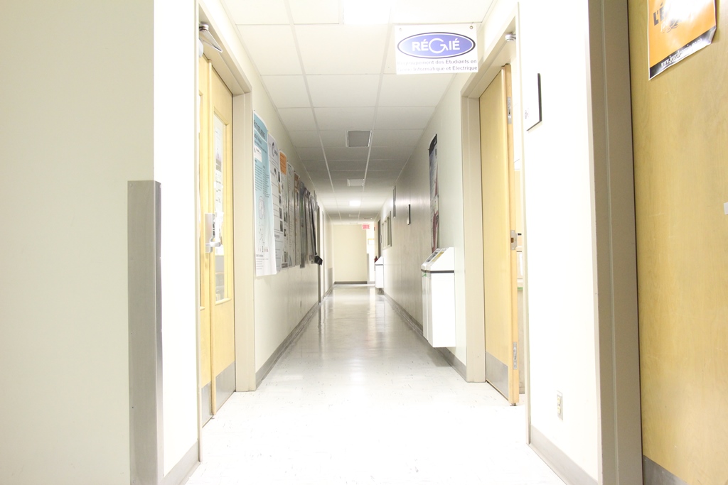
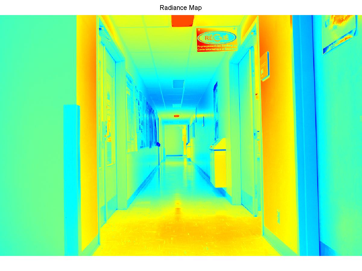
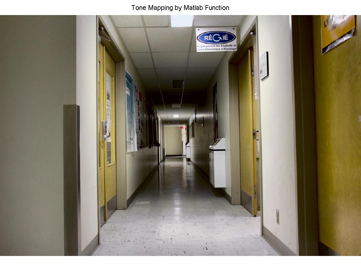
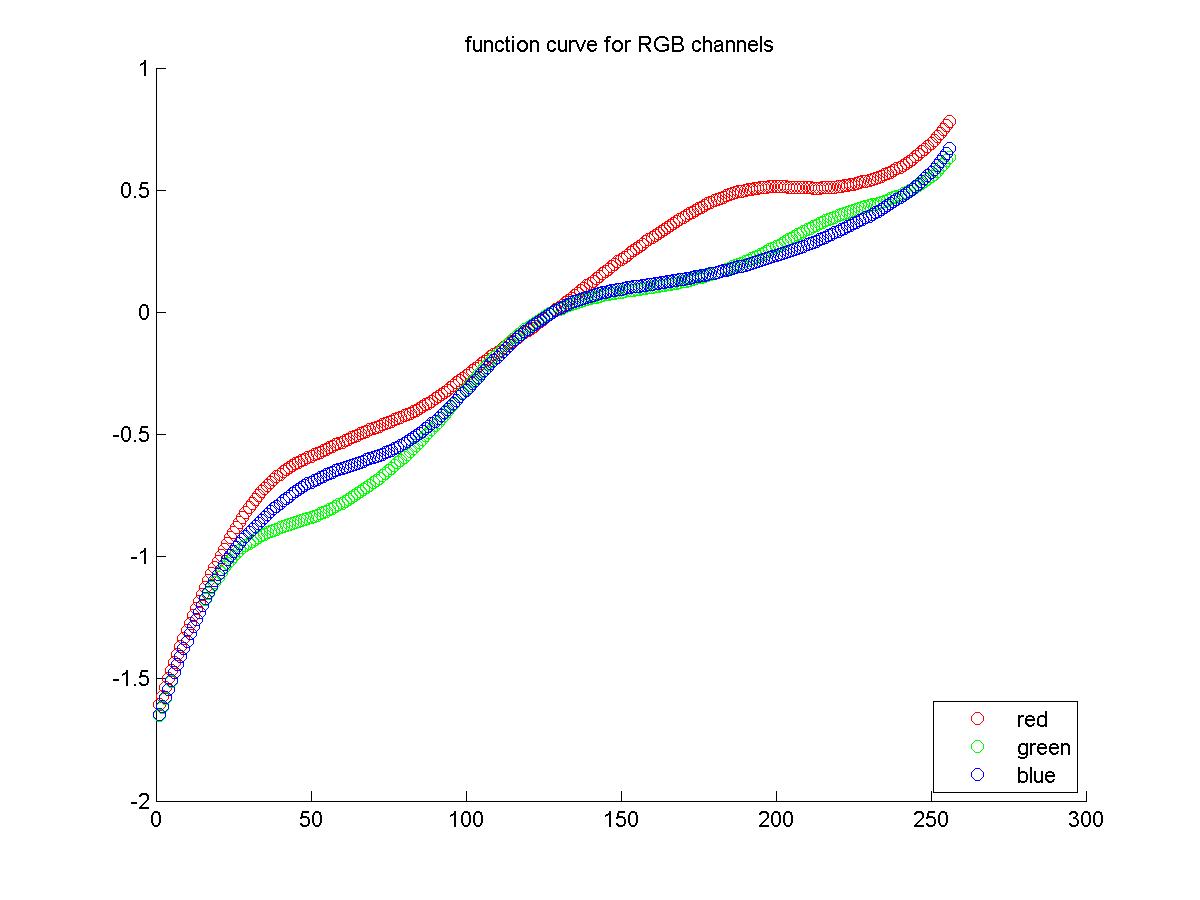
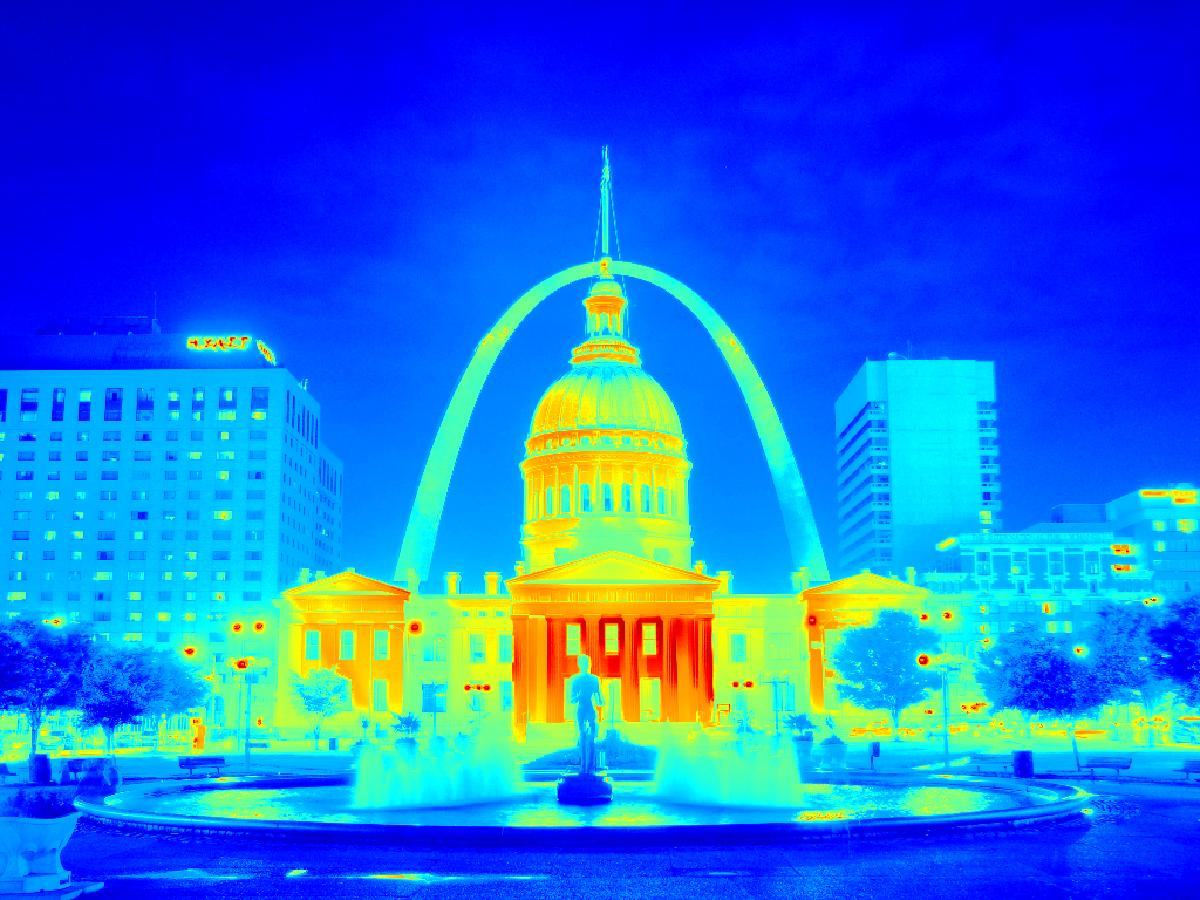
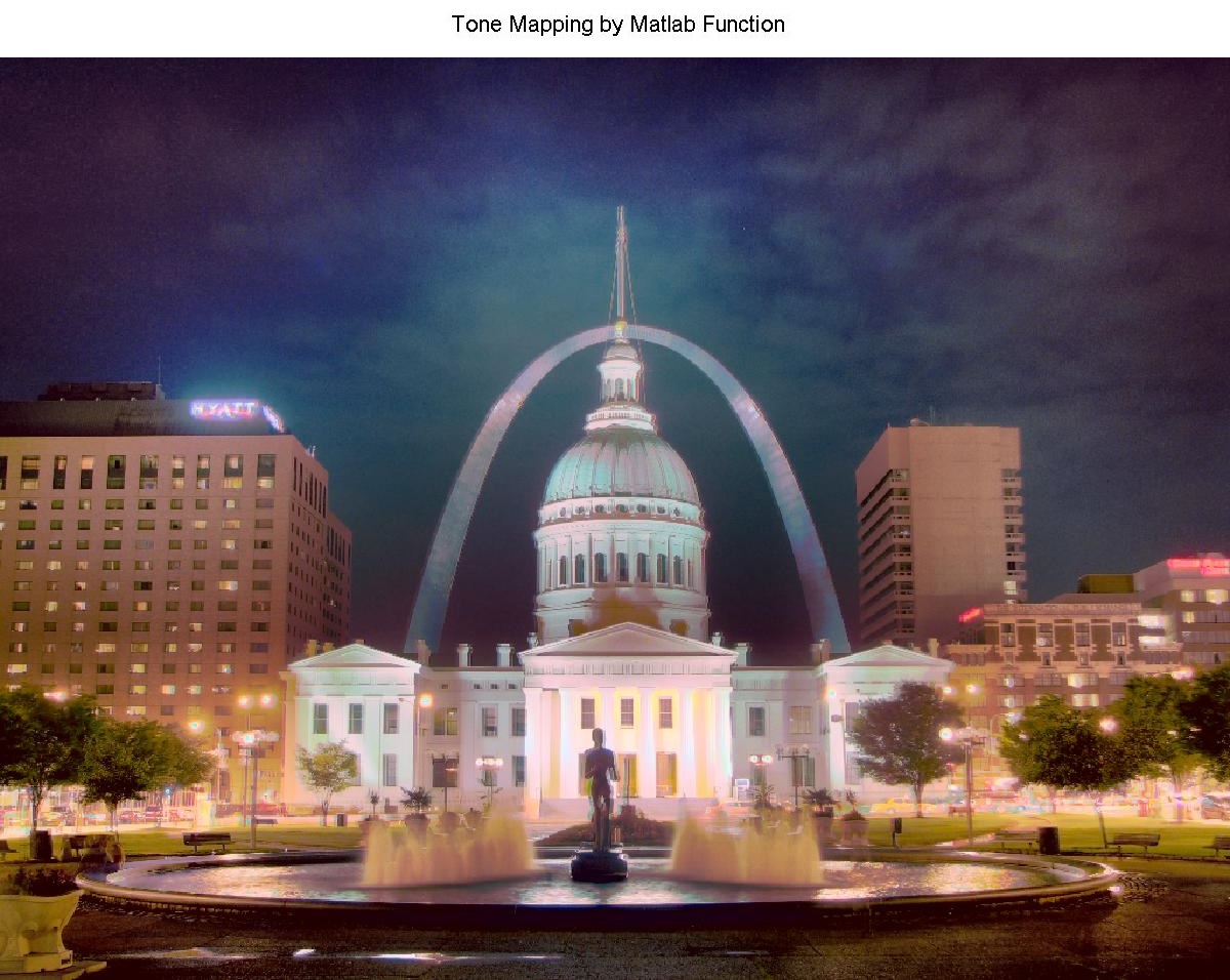
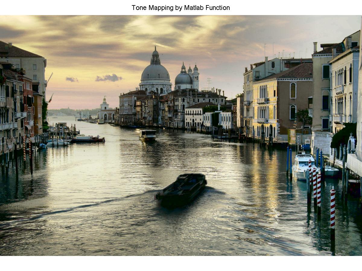
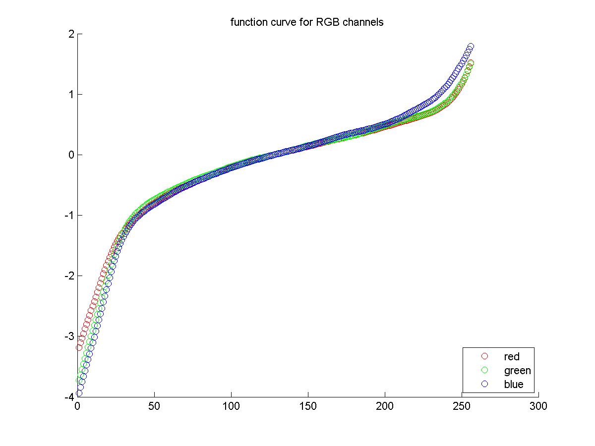
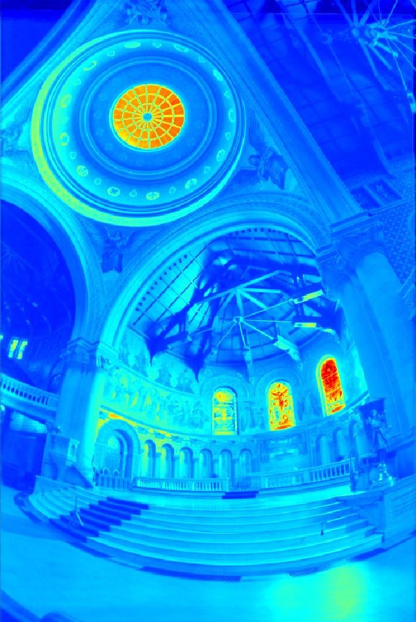
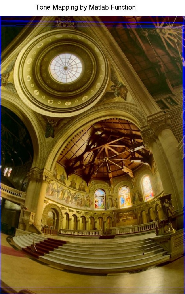
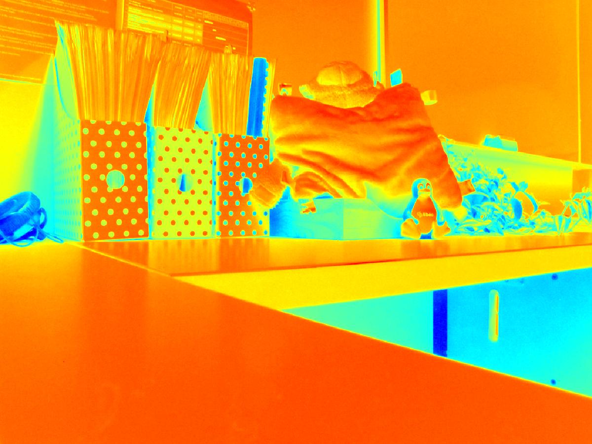
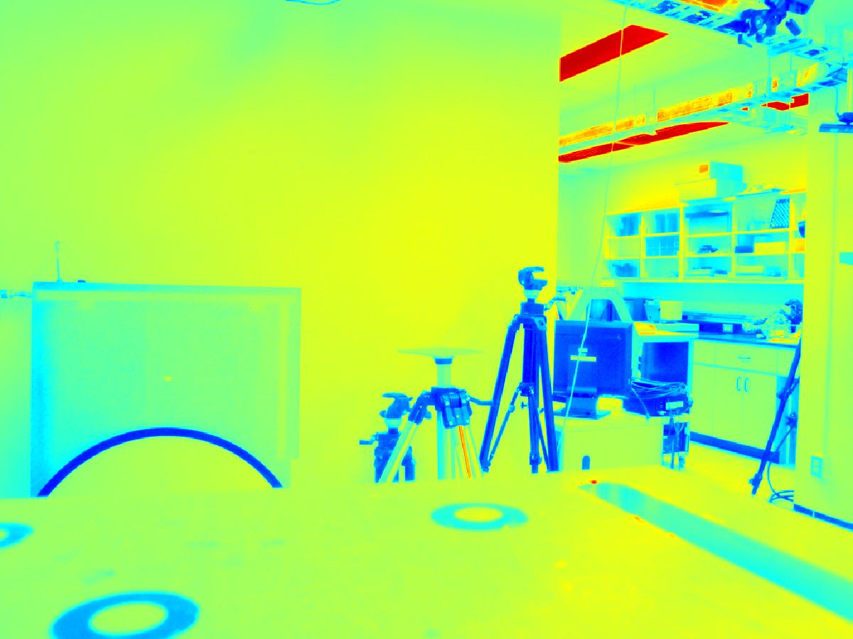
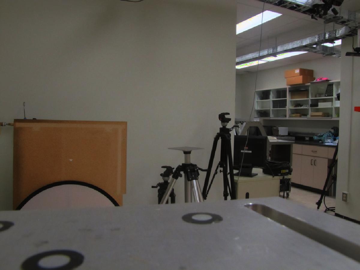
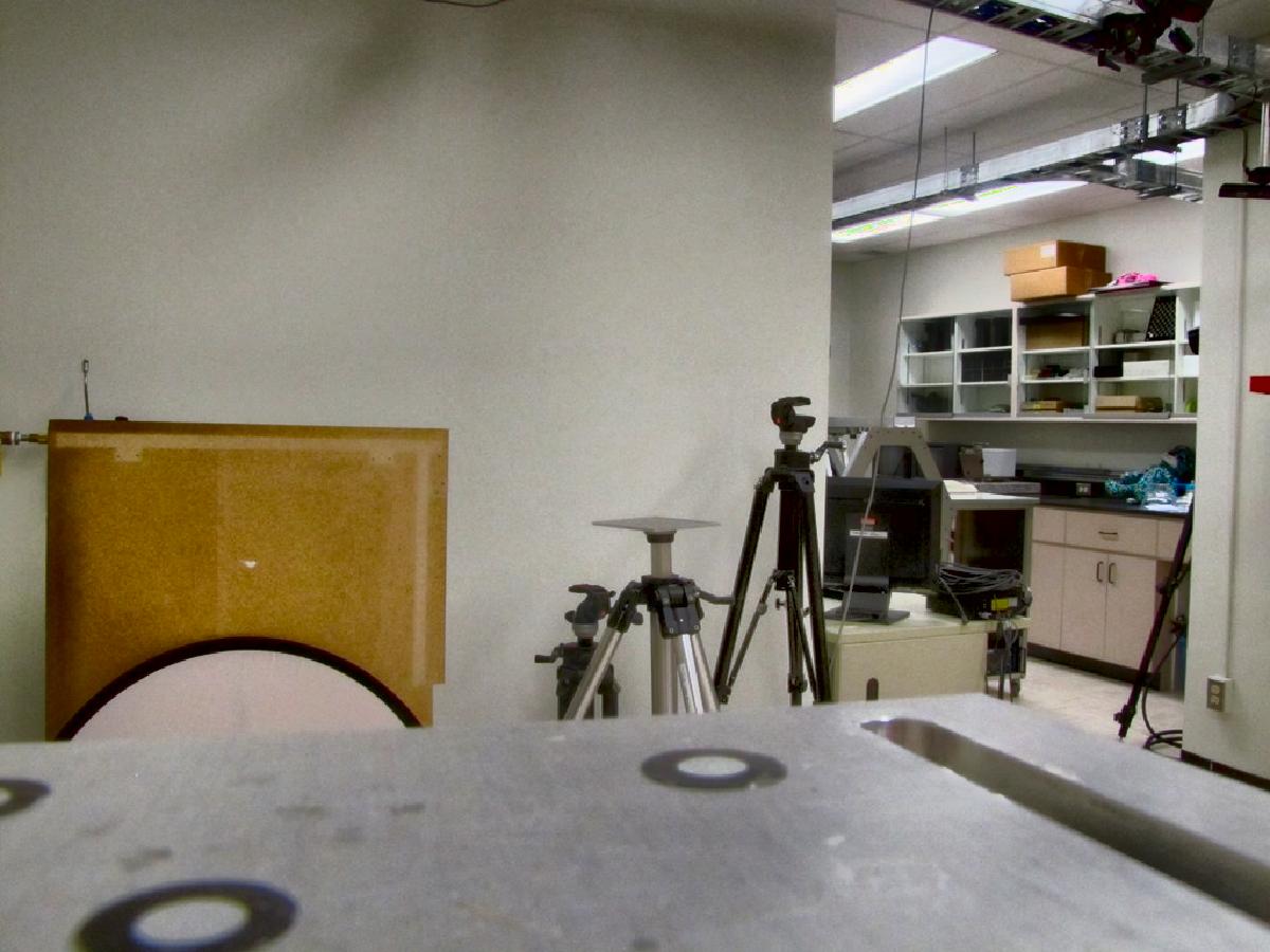
Here we have a plot of the g function, a color visualization of the radiance map generated by the algorithm and I've also included the result of the image, for comparison to the radiance map.
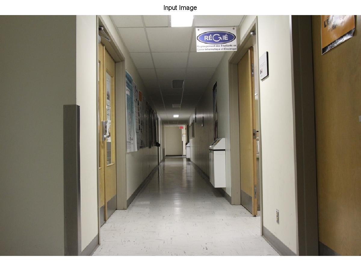
1- Corridor set
2- Stlouis set
3- Grandcanal set
4- Debevec set
4) Bells and Whistles
4.1 - Use other images!
Here we tried our code over various set of images.
1- Nature set
2- Libarary set
3- Office set
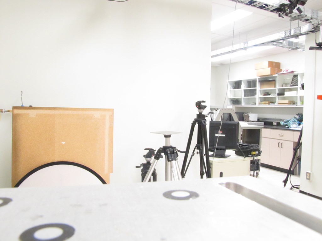
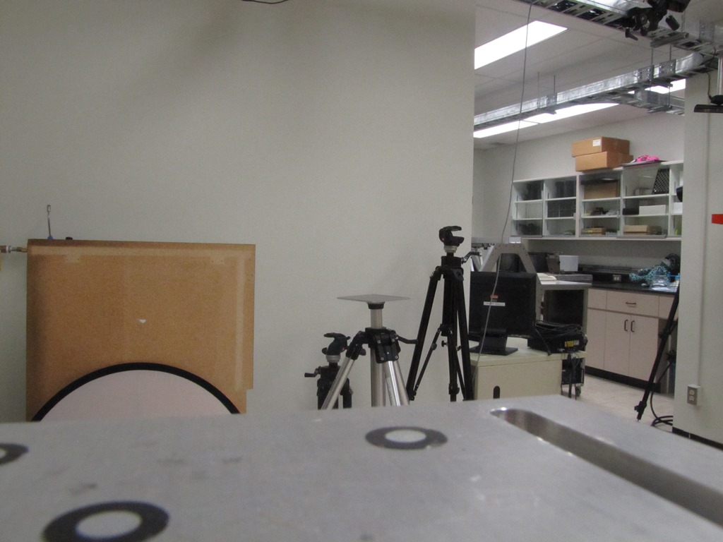
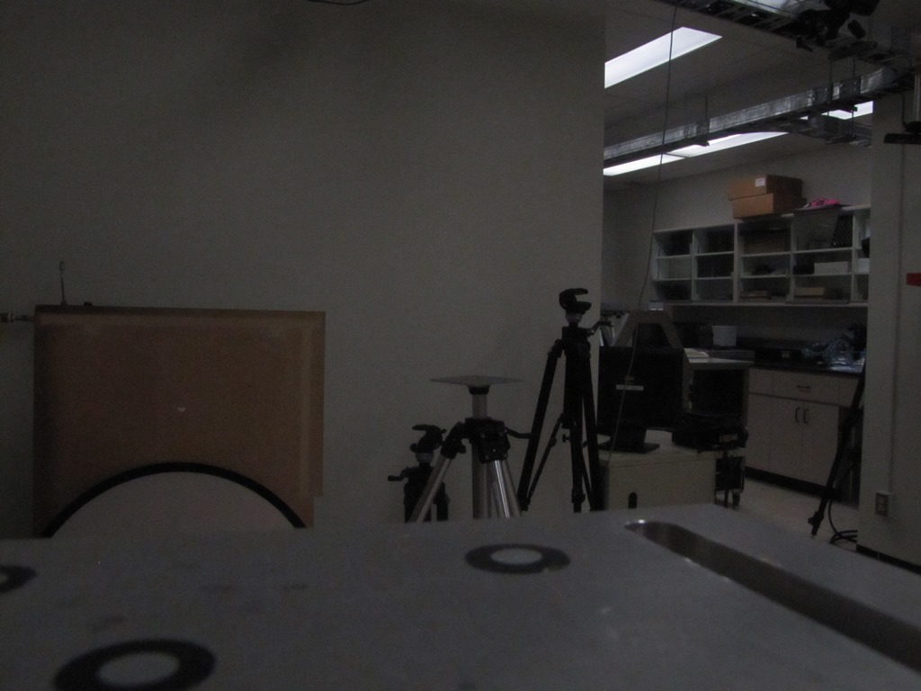
3- Vision Lab set
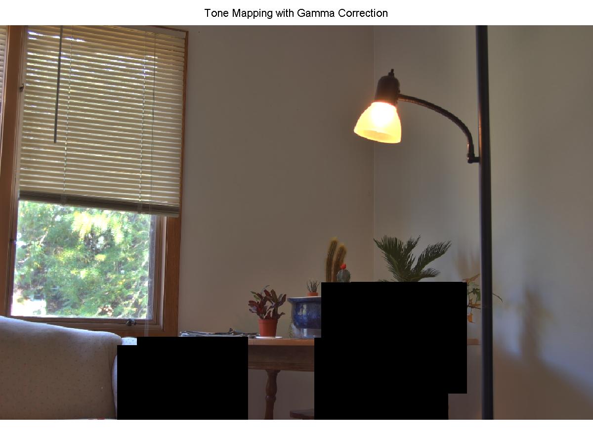
In the following results you can observe some black spots.
1- Apartment set
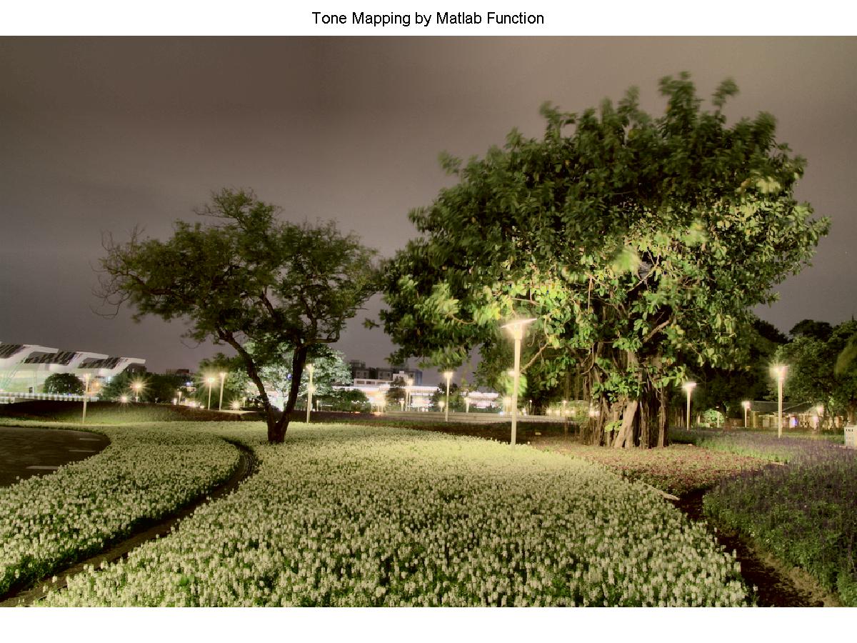
2- Tree set
It is because HDR images have zero values which will cause problems with log and we can fix this problem by replacing all either NAN or INF by the smallest non-zero values. You can see the affect in the following figures
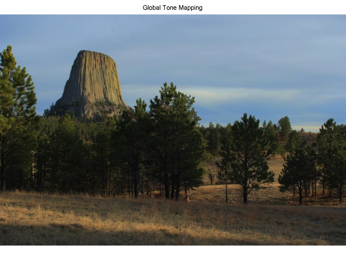
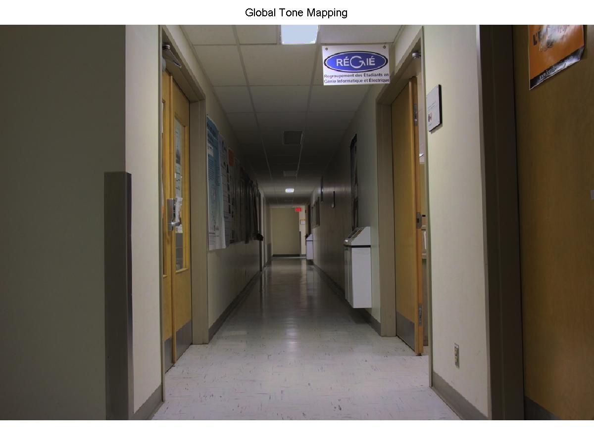
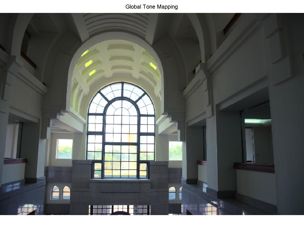
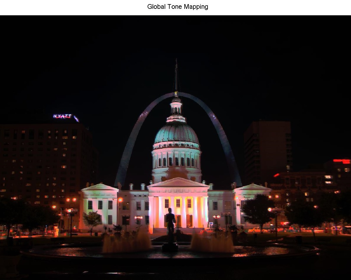
4.2 - Global Operator !
We also implement a simple global operator, using Lnew = L / (1+L). Here, We want to show some of the results. It includes a parameter b that can be adjusted according to the desired brightness in the final image.
Global tone mapping does not always work or give a goog result. For instance, In following image you can see the difference between global tone mapping and local tone mappingthat. Local mapping did this job better than global mapping.
4.3 - Fast Bilateral Filtering using "sub-sampling" !
Downsampling the 3D space before applying filter Bilateral filter does not makes a considerable difference in the accuracy but increases speed. It can be done in 3 step :
1) Downsample the image and build a 3-D space grid
2) Compute the convolution between the new grid
3) Interpolate the values and get the final blurry results
I tried but unfortunately, I could not solve the problem with my code and demonstrate the result relevant to this part.