Project Description
The real world has a very high dynamic range. However, the photo taken by modern camera can often only capture a small part of range, which usually suffers from either over-exposure or under-exposure for the scene with high dynamic range. The solution to this problem is first to take multiple images of the same scene with different exposure time. With these images, a mapping from each pixel value to a specific radicane can be established, which results in a 'radiance map'. Having obtained the radiance map, several 'tone mapping' methods can be applied to compress the radiance map into a displayable range. In general, tone mapping consists of global and local techniques.
Algorithm Inplementation
Part 1: Radiance Map Construction
The construction of radiance map [see the code 'construct_radiance_map.m'] based on the idea of [Debevec and Malik 1997] mainly consists of two steps: The first step is to identify the response curve 'g' that maps the pixel values to the log of exposure values for three seperate color channels [see the code 'g_curve.m']. Once the curve 'g' is available, the second step is to map the observed pixel value and exposure time in the exposure image set to the radiance for each pixel using the weighting fuction 'w' [see the code 'HDR_radiance_map.m']. Before the two mian steps, a point-selecting step is performed to automatically randomly select sufficient number of pixels that are evenly distributed from range 0 to 255 [see the code 'select_pixels.m'].
Result of Radiance Map Construction
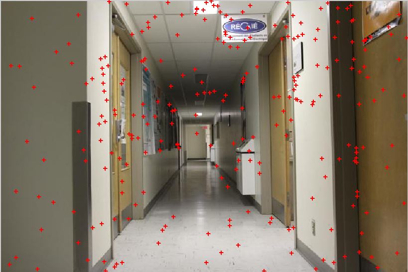
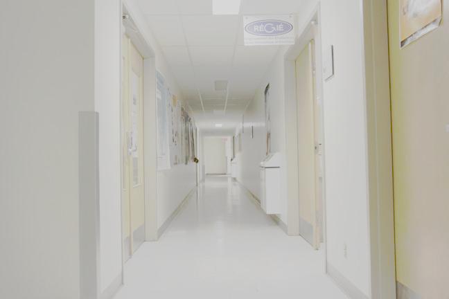
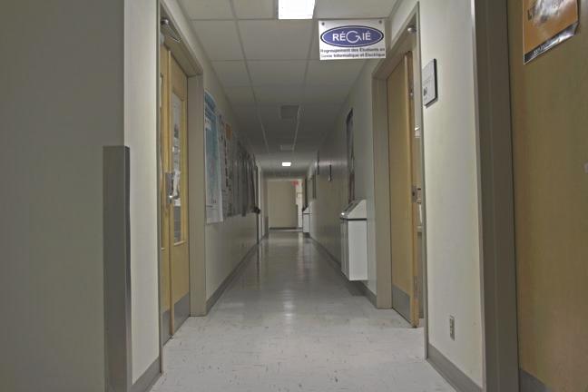
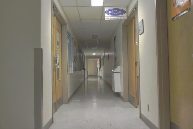
The number of selected pixels must satisfy the condition 'N(P-1) > 256' suggested in the paper. An exmaple is illustrated as below with 'N=260' and 'P = 3' for the 'corridor' set. we can see that the points are uniformly distributed in the intensity range as well as space.
| the automatically selected pixels for 'corridor' image set |
 |
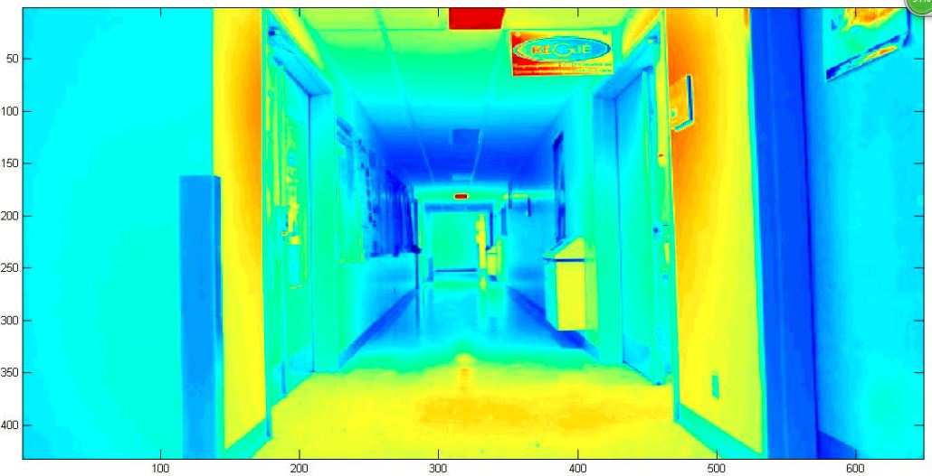
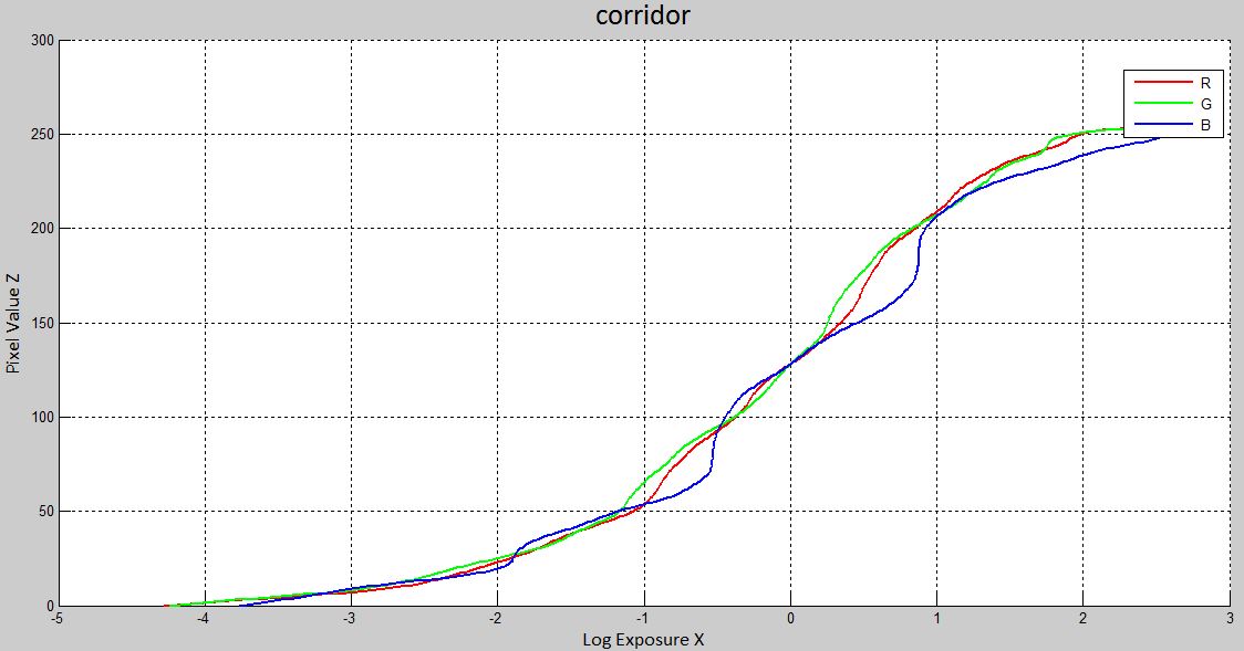
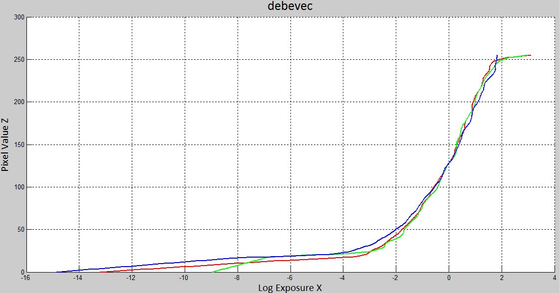
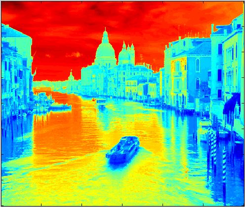
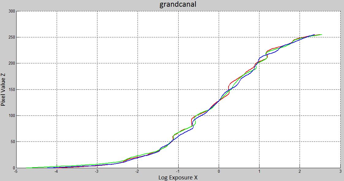
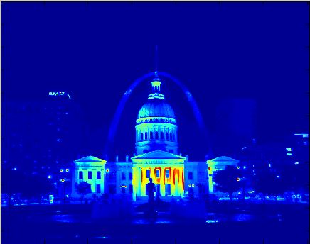
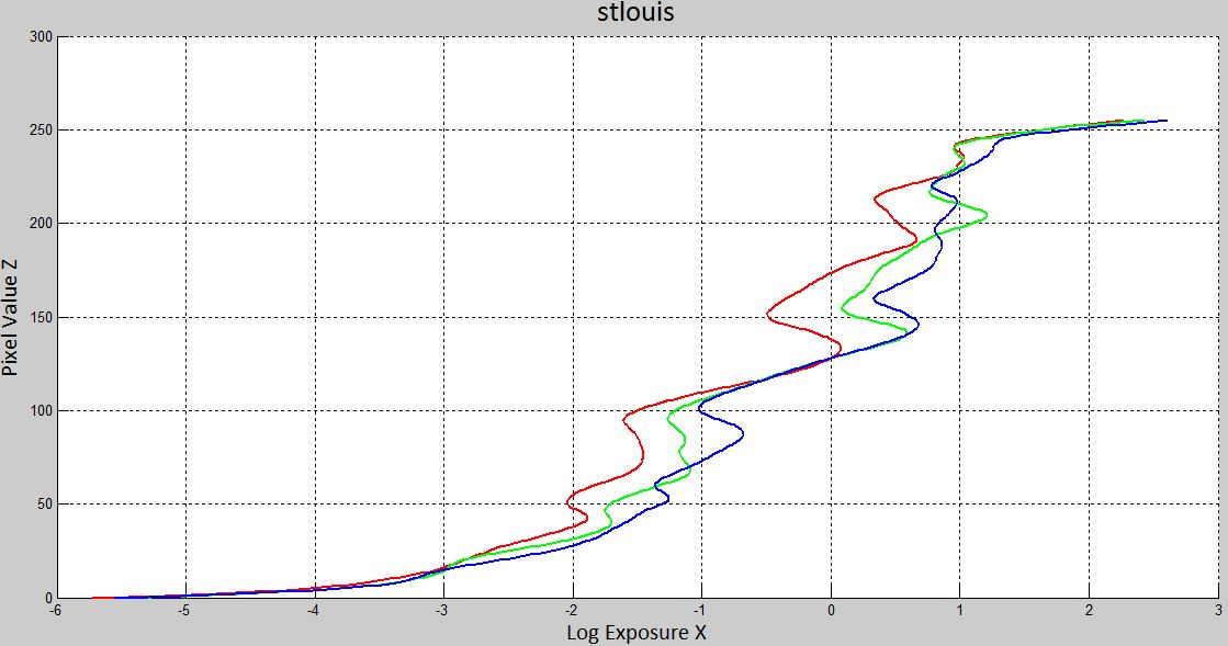
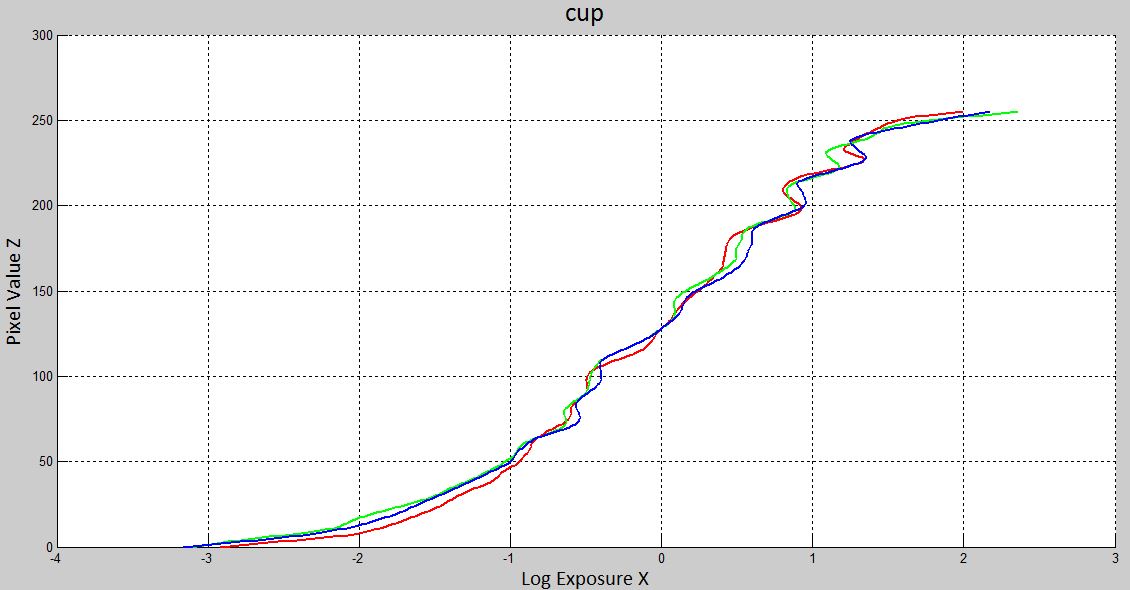
The reconstructed radiance maps are shown on the left and the response curve are shown on the right
| Radiance Map | Recovered response curves |
 |
 |
 |
 |
 |
 |
 |
 |
Part 2: Tone Mapping
In the second part of the pipeline, the resulting radiance map is need to compressed by a tone mapping operator so as to fit into the displayable range (0 to 255). In general, there are two class of tone mapping methods. One method from global tone mapping class is to calculate the pixel value for each radiance value L to be 'L / (1+L)' [see the code 'global_simple_tone_mapping.m']. However, the result of global operator is not satisfactory since the details of both brighter and darker regions can not be distinguihed very well at the same time. To tone map locally, we inplement the idea of [Durand 2002] that is based on a bilateral filtering on a separatable low-frequency layer. Specifically, the method contains the following steps: [see the code 'durand_tone_mapping']
(1) separate the intensity image from the color components and the intensity is compressed into the log domain.
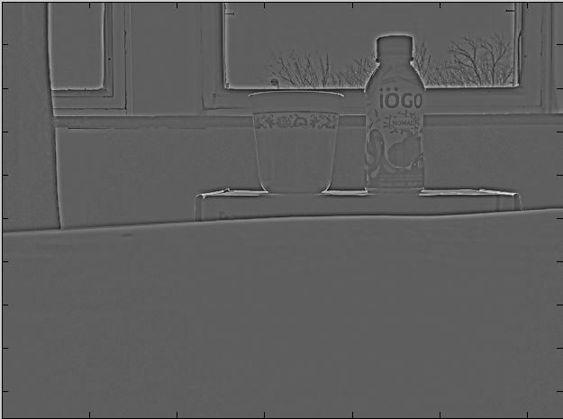
(2) divide the intensity image into the detailed and large-scale components. To do this, we first obtain the large-scale layer by bluring the intensity image using a edge-preserving bilateral filter which takes both spatial and intensity range into consideration at the same time [see the code 'bilateral_filter.m']. Then, the detailed layer can be recovered by subtracting the blurred large-scale layer from the intensity image.
(3) the large-scale layer is compressed in order to reduce the contrasts while keeping the other components intact.
(4) the compressed large-scale layer, the detail layer and the color layer are recombined to form the HDR image.
(5) a gamma correction is used to ajust the final HDR image.
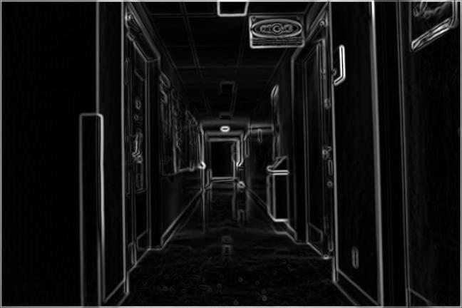
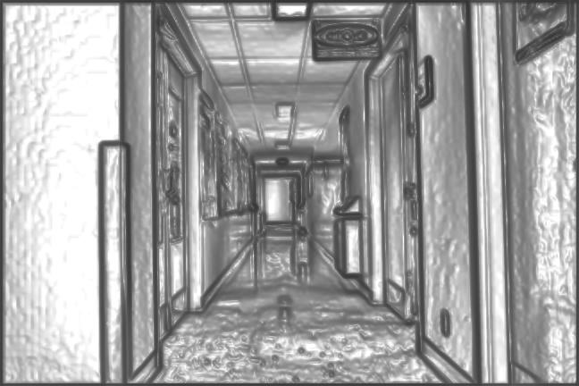
Result of Bilateral Filtering of Tone Mapping
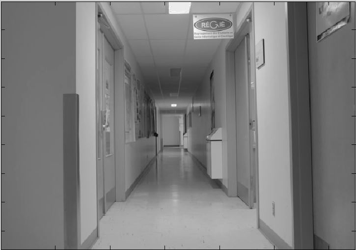
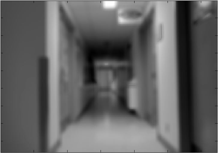
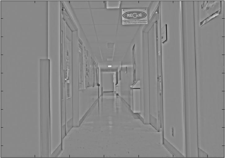
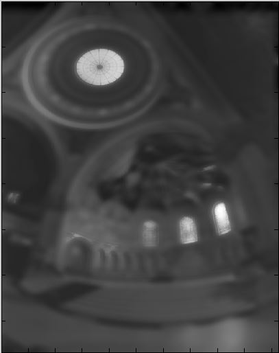
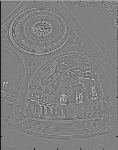
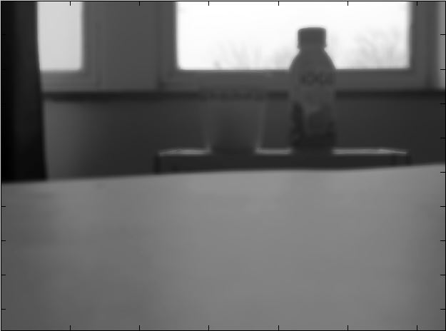
The sigma parameter for the spatial Guassian filter and range Guassian filter is 10 and 4, respectively. The base layer and the detail layer are shown below.
| Intensity | Base after bilateral filtering | The detail layer |
 |
 |
 |
 |
 |
 |
 |
 |
 |
 |
 |
 |
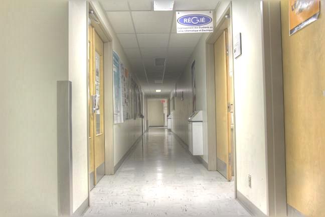
Result of Reconstructed HDR
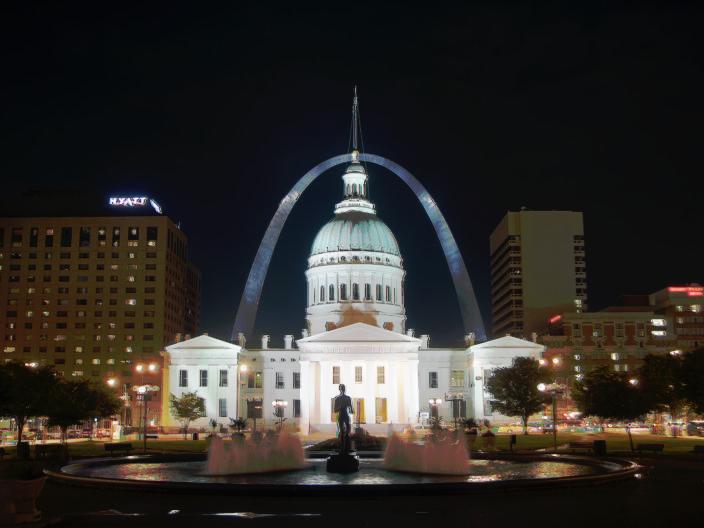
| GLobal | Durand |
 |
 |
 |
 |
 |
 |
 |
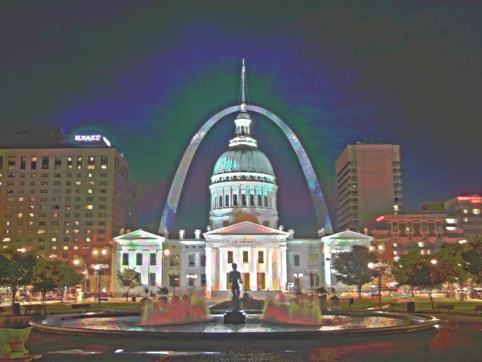 |
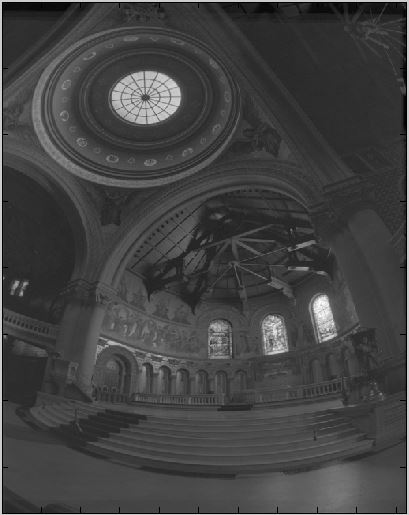
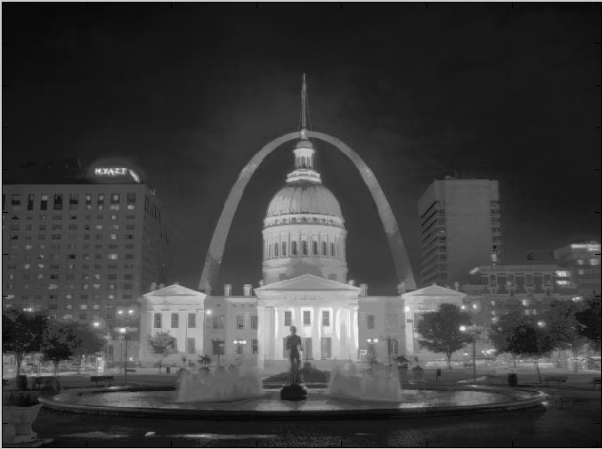
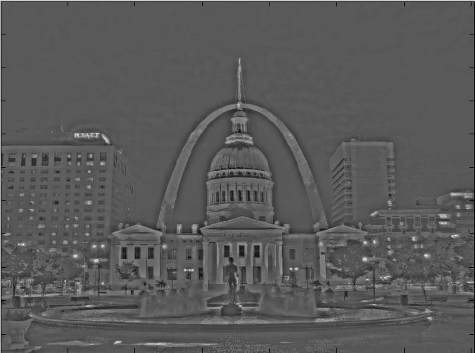
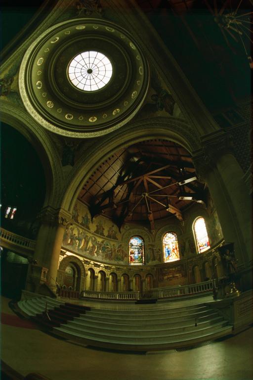
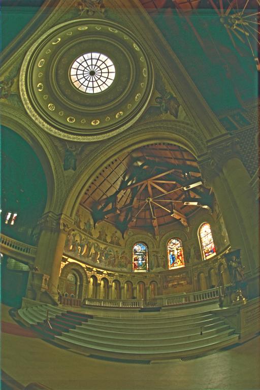
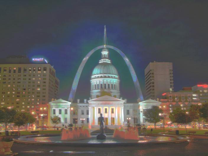
As we can observe from the above results, the local method is obviously better than the global method since the latter reveals more details on both under-exposure and over-exposure regions. However, the result of 'debevec' image is not as good as I expected, the structure of ceiling in darkest region is supposed to be discerned. Maybe I have not completely successfully implement the brutal force algorithm, or maybe the parameters of Guassian filters need to be appropriately ajusted.
Bells and Whistles
(1) Using My Own Image
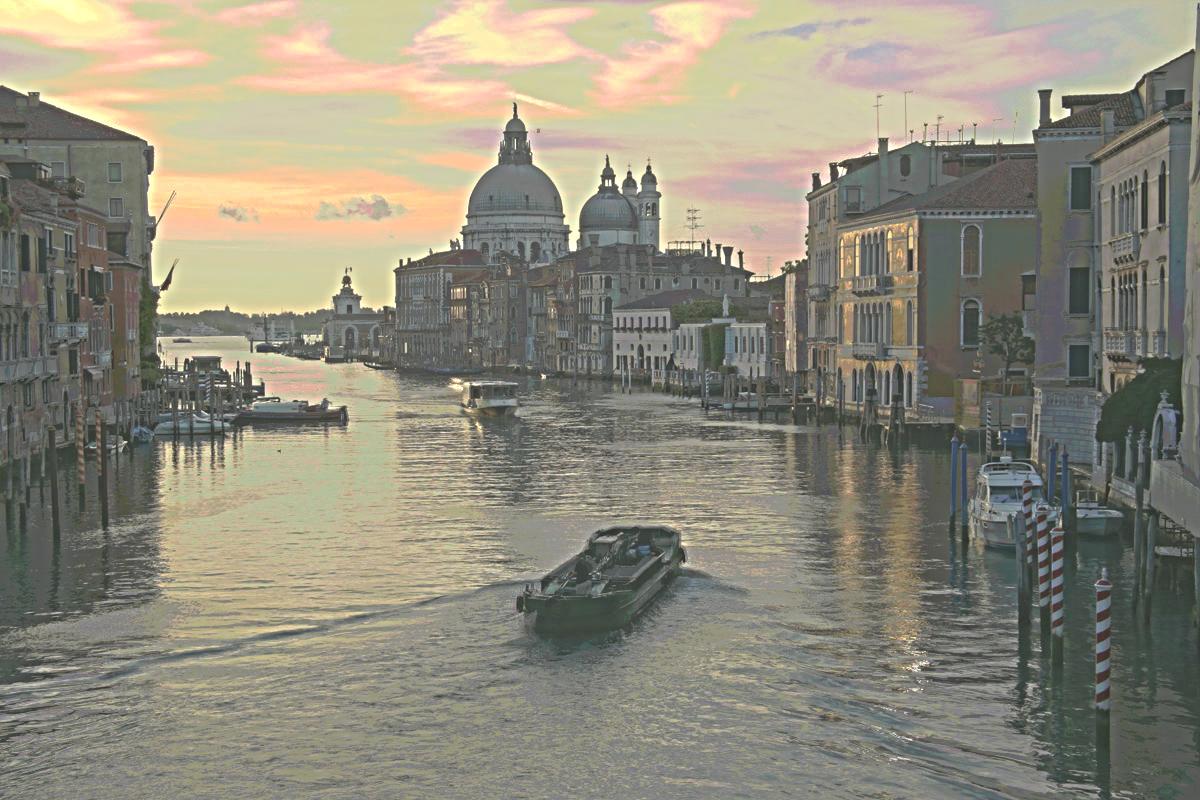
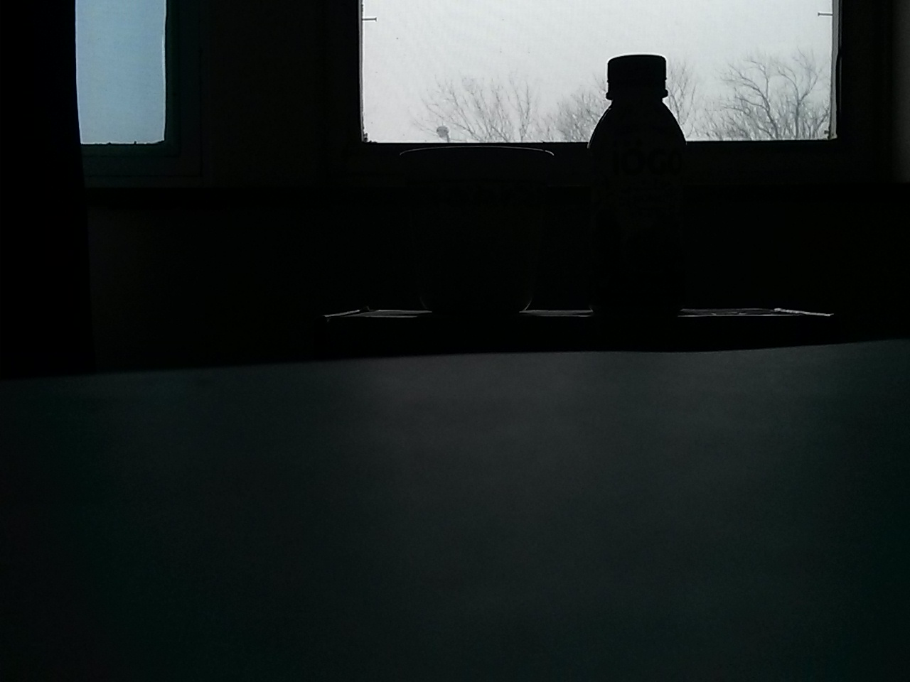
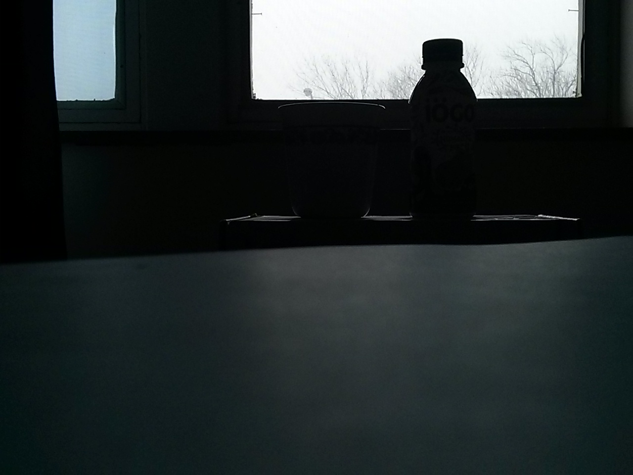
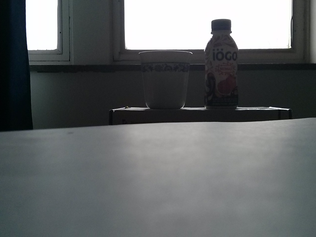
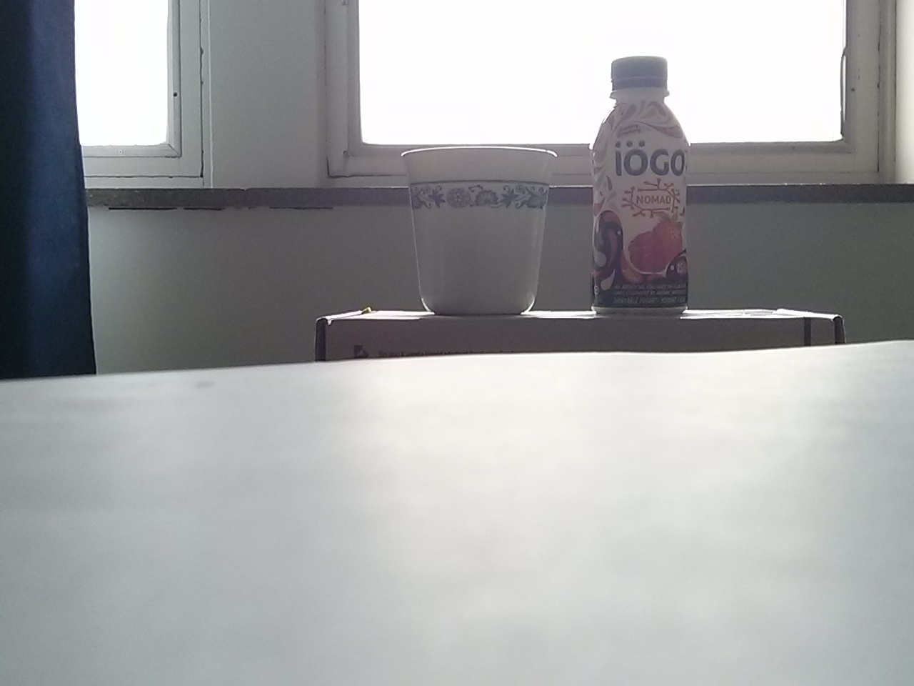
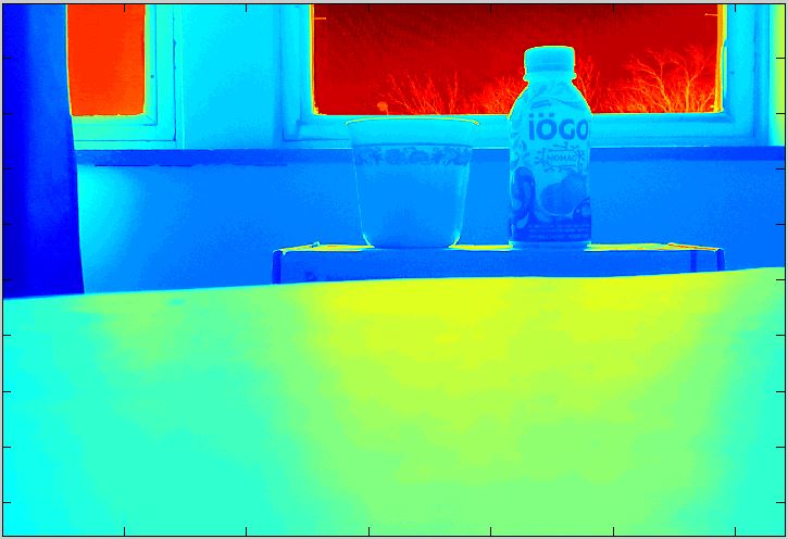
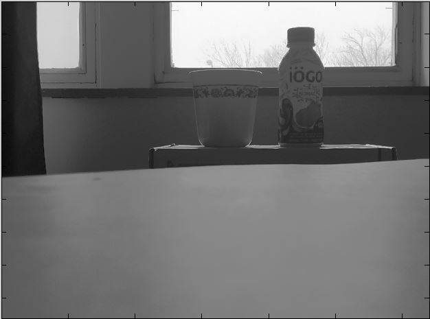
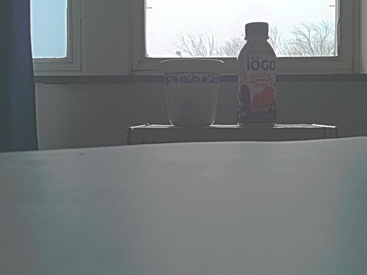
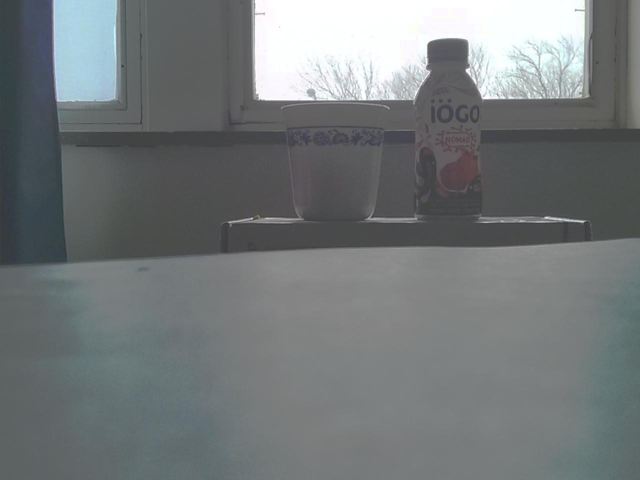
The sequence of photoes I use have the different exposure time ranging from 1/438 to 1/30 second. Such image set with an indoor-outdoor scene suggests an very high dynamic range. And a HDR image is successfully recovered from this set by local tone mapping, scine both the details of the bottle and the structure of the tree can be easily seen at the same time from the resulting HDR image.
| 1/438 second | 1/271 second | 1/100 second | 1/30 second |
 |
 |
 |
 |
| Radiance Map | Recovered response curves |
 |
 |
| Intensity | Base after bilateral filtering | The detail layer |
 |
 |
 |
| GLobal | Durand |
 |
 |
(2) Fast Bilateral Filtering
In order to speed up the bilateral filtering, another bilateral filtering method is implemented according to the work of [Paris and Durand 2006] by treating the intensity image as the third dimension and reformulate the bilateral filter as a 3D gaussian convolution followed by simple nonlinearities. The key idea that accelerates the computation is computing the 3D convolution at a coarse resolution, this is done by a downsampling procedure and then followed by an upsampling procedure [see the code 'fast_bilateral_filter.m'].
Result of Fast Bilateral Filtering
| size of image | brutal bilateral filter | fast bilateral filter |
| "corridor" of 432 x 648 | 215.75 seconds | 0.18 seconds |
| "debevec" of 512 x 768 | 307.40 seconds | 0.22 seconds |
| "grandcanal" of 800 x 1200 | 1234.40 seconds | 0.52 seconds |
| "cup" of 960 x 1280 | 1471.20 seconds | 0.67 seconds |
We can see from the table that the fast bilateral filter can filter an intensity image within one second. In contrast, the brutal bilateral filter for the image sets shown in the table is at least a thousand times slower than fast bilateral filter. In the case of image set with larger size, the gap will be more significant. The following constructed HDR images are produced by brutal bilateral filter (left) and fast bilateral filter (right).
| brutal bilateral filter | fast bilateral filter |
|
 |
|
 |
|
 |
|
 |
Using the 3D space, it has been proven that the convolution computation can be downsampled without significant impact on the resulting accuracy. The above results show that fast method are comparable with the brutal method, and we can see the images of fast method are a little bit blurred and dark than the brutal method.
(3) Gradient Domain Tone Mapping
In this part, I implement the full version of the local tone mapping method from [Fattal 2002]. Generally speaking, this simple method relies on the assumption that the HDR image must give rise to large magnitude gradients at some scale. Therefore, they identify the large gradient at various scales levels, and progressively attenuate their magnitudes so as to compress the significant luminance changes while preserving the details. At last, a LDR image is reconstructed from the attenuated gradient field by solving a Poisson equation. Specifically, it can be implemented by following steps: [see the code 'gradient_domain_HDR.m']
(1) separate the intensity image from the color components and the intensity is compressed into the log domain.
(2) compute the gaussian pyramid. At each level of the pyramid, the intensity is first blurred by a guassian filter, then the gradients are calculated on the filtered intensity [see the code 'gradient_gaussian_pyramid' function].
(3) compute compute the gradient attenuation matrix 'Phi'. Starting from the top level, the scaling factor 'phi_k' for attenuation of a specific level is propagated to the next level using linear interpolation, and the overall attenuation matrix 'Phi' is accumulated to the finest bottom level [see the code 'gradient_attenuation_matrix' function].
(4) apply the accumulated matrix 'Phi' to attenuate the gradients of the finest level to obtain the attenuated gradient 'gx' and 'gy' [see the code 'gradient_attenuation' function].
(5) solve for the intensity image whose gradients are the approximation of 'gx' and 'gy' by a Possion equation.
(6) combine the color component and the compressed intensity imageto form the HDR image.
Result of Gradient Domain Tone Mapping
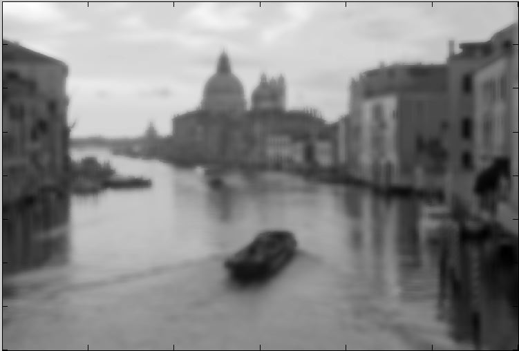
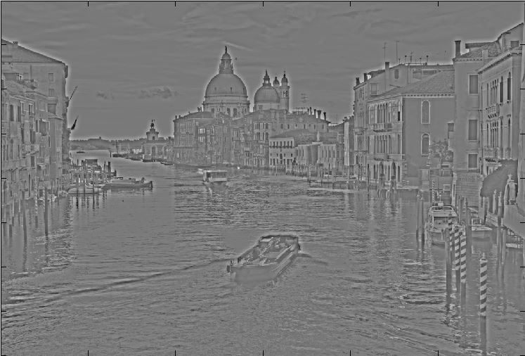
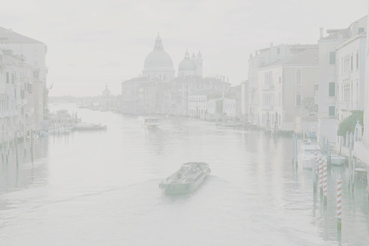
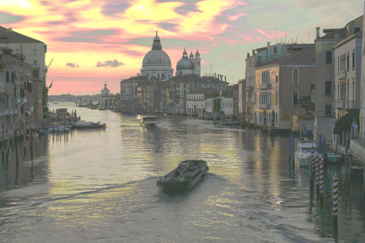
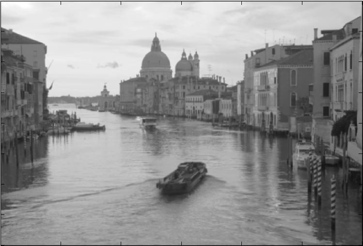
Fristly, I will take the 'grandcanal' set as an example to illusrate the result of gradient domain tone mapping. In this implementation, the paramter 'alpha' that determines which gradient magnitude to attenuate is chosen to be 0.1 times the average gradient magnitude. The parameter 'beta' representing the degree of attenuation is set as 0.85. The number of Guassian pyramid layer is 3.
The images below correspond to the three layers of Guassian pyramid with factor of 2. I use a 5x5 Guassian fitler to blur the intensity image before downsampling.
| the 3rd layer 200x300 | the 2nd layer 400x600 | the 1st layer 800x1200 |
 |
 |
 |
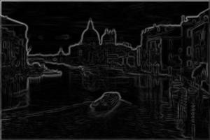
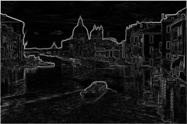
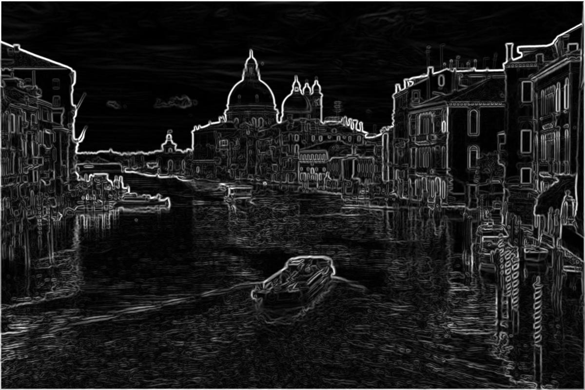
The gradients of each layer are shown as below.
| gradients of the 3rd layer | gradients of the 2nd layer | gradients the 1st layer |
 |
 |
 |
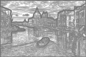
The accumulated gradient attenuation matrix 'Phi' for the three different layers from top to bottom are demonstrated from left to right. The darker shades indicates the stronger attenuation, and we can see that the degree of attenuation propogates from coarsest layer to finest layer.
| Intensity | Base after bilateral filtering | The detail layer |
 |
 |
 |
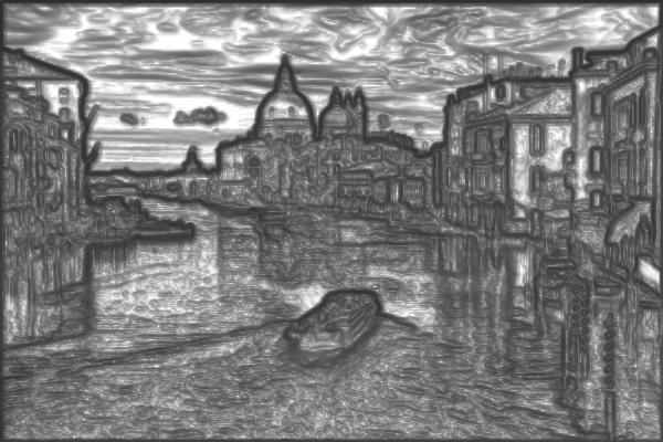
The image is on the left is constructed from gradients of the original image, and the right image corresponds to the attunuated image whose gradients with larger magnitude are significantly compressed.
| gradients before attenuation | gradients after attenuation |
|
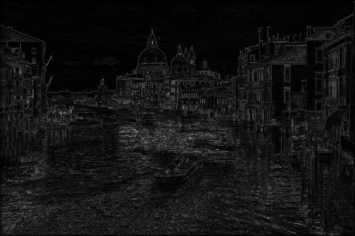 |
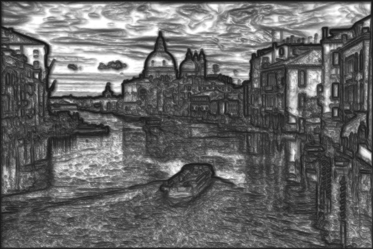
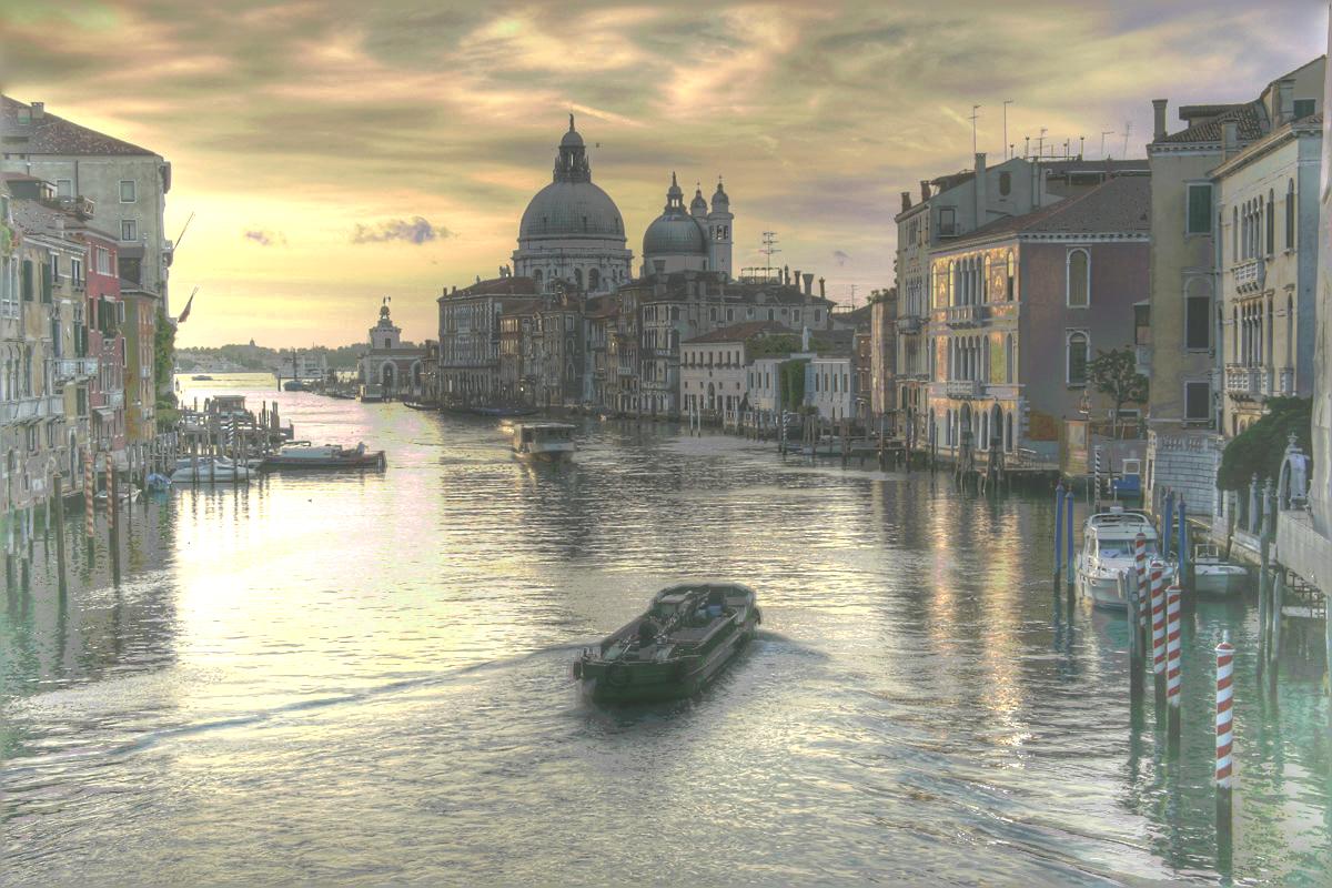
Comparing with the brutal force Durand method, the gradient domain method is conceptly simple and computationaly efficient as well. The resulting compressed HDR image (right) can be obtained in less than one second, which is much faster than the brutal force Durand tone mapping. Furthermore, the gradient domain method gains a better performance in that more details can be distinguished. e.g. The details of cloud in the brighter sky can be captured by the right image.
| brutal force Durand tone mapping | gradient domain tone mapping |
|
 |
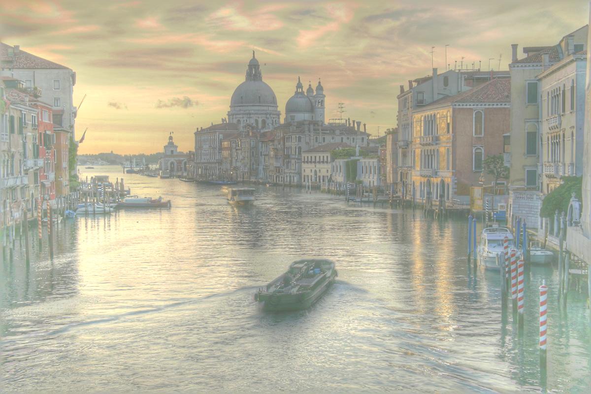
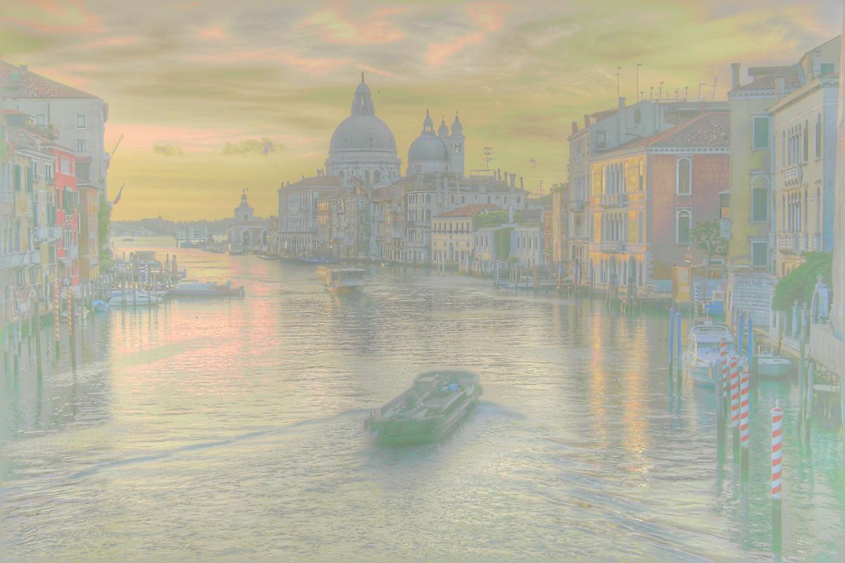
Another important factor for achieving a better performance is to choose the appropriate number of pyramid layers. The following results corresponds to 2, 3 and 4 layers of pyramid, respectively. The 4 layer result shows that the contrast range is compressed too much by accumulating the attenuation of gradients from 4 different sacles.
| with 2 layers | with 3 layers | with 4 layers |
 |
 |
 |
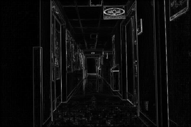
The following images is the result of 'corridor' image set. The first row is the original gradients, attenuation matrix and the attenuated gradients. The result from the brutal force Durand and gradient domain are listed in the second row.
| the original gradients | the attenuation factor | the attenuated gradients |
 |
 |
 |
| brutal force Durand tone mapping | gradient domain tone mapping |
|
 |