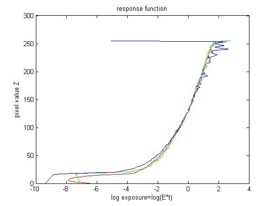
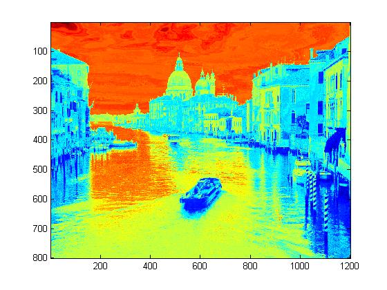
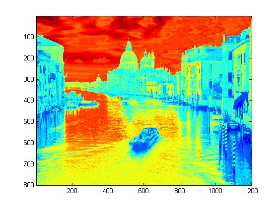
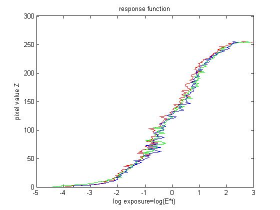
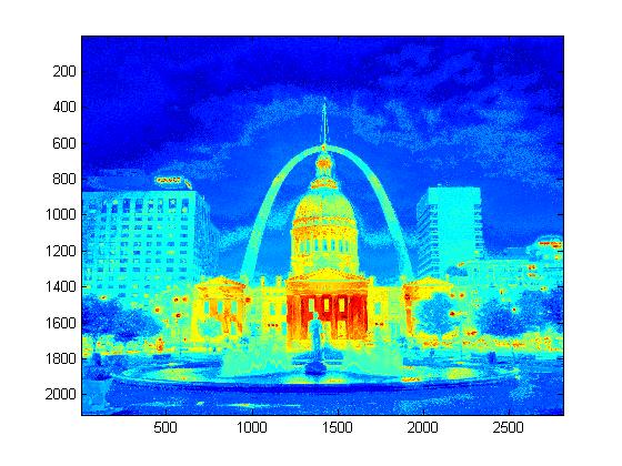
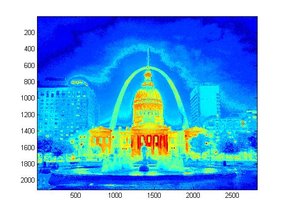
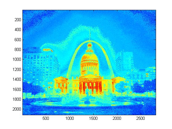
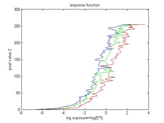
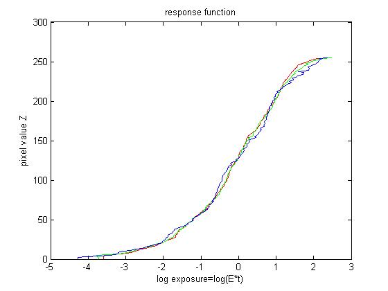
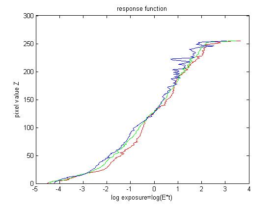
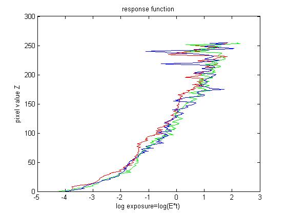
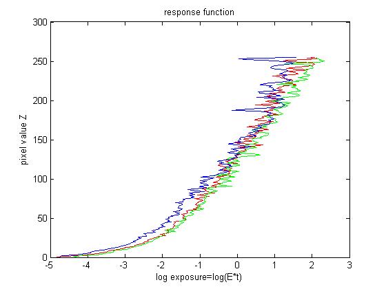
To recover the response function between pixel values and real radiance, we need several images of different exposures of the scene radiance. For each image, I choose randomly around 1000 positions and obtain the corresponding R G B values. The observed pixel value \(Z_{ij}\) for pixel \(i\) in image \(j\) is a function of unknown radiance \(E_i\) and known exposure duration \(\Delta t_j\), i.e. \(Z_{ij}=f(E_i*\Delta t_j)\). I solve the inverse function of \(f\) in log domain, i.e. \(g=ln(f^{-1})\). This function \(g\) maps from pixel values (0~255) to the log of the exposure values: \[g(Z_{ij})=ln(E_i)+ln(t_j)\] This leads to construct a group of linear equations \(Ax=b\). Furthermore, g is assumed to be monotonic and smooth, so we need impose constraint on g. So we add some penalizing term to the group of equations, i.e. \[g''=(g(x-1)-g(x))-(g(x)-g(x+1))=g(x-1)+g(x+1)-2*g(x)\]. After that a lambda is assigned to each smooth part and a weight function based on pixel value is assigned for different \(g\). Finally, I solve this overdetermined linear equation systems using least square method.

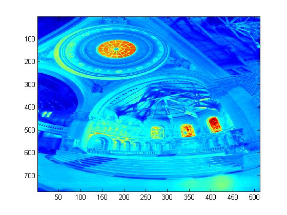
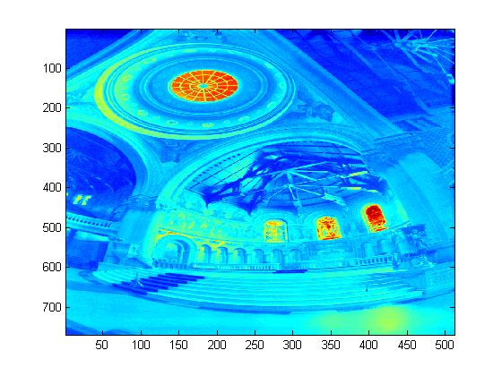
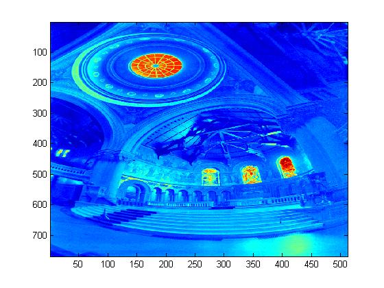
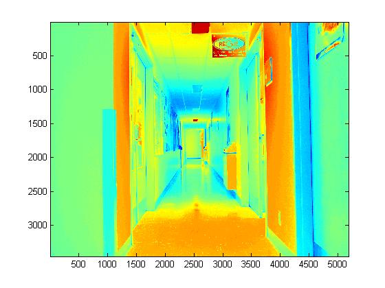
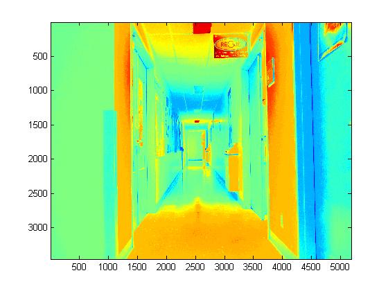
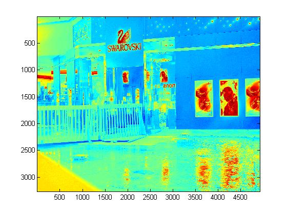
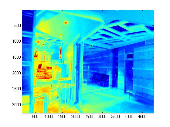
After we have the response function \(g\), we can compute the radiance map for each corresponding pixel in a straightforward way. To get a better result, the weight function is needed, i.e.\[ln E_i=\frac{\Sigma_{j=1}^{P}w(Z_{ij})(g(Z_{ij})-ln \Delta t_{j})}{\Sigma_{j=1}^{P}w(Z_{ij})}\]

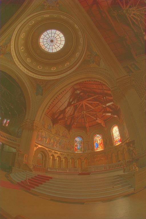
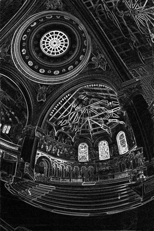
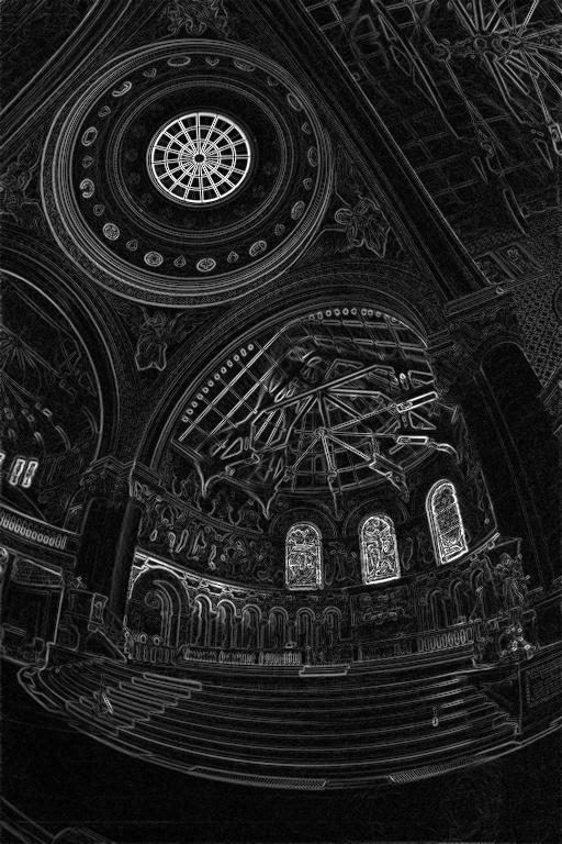
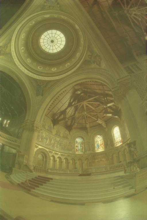
Experimental Results for Radiance Map Construction

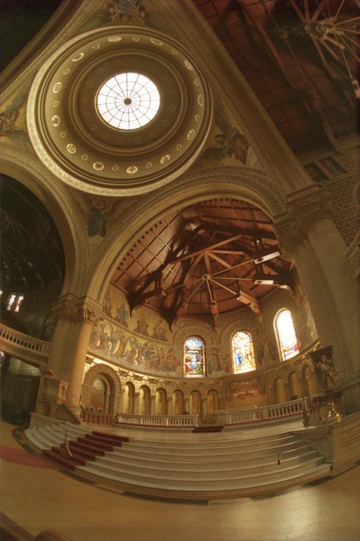
Part 2: Tone Mapping

After we get the radiance map, the next job is to display the HDR image on a LDR device in a suitable way. Tone mapping is a technique used to map one set of colors to another in order to approximate the appearance of high dynamic range images on dynamic limited medium since for a computer it can only save color intensity using 8-bit bytes. There are two categories of tone mapping method. One is global tone mapping , the other is local tone mapping.

Global Tone Mapping

For global tone mapping, I choose the trivial function \[V_{out}=\frac{V_{in}}{V_{in}+1}\], where \(V_{in}\) is the luminance of the original pixel and \(V_{out}\) is the lunminance of the filtered pixel. This function will map \(V_{in}\) in the domain\([0,\infty]\) to \(V_{out}\) in the domain \([0,1]\).

Local Tone Mapping

For this part, I implement the bilateral filtering method as professor asked. A bilateral filter is a non-linear, edge-preserving and noise-reducing smoothing filter for images. The intensity value at each pixel is computed by a weighted average of intensity values from nearby pixel. The output of the bilateral filter for a pixel s is defined as following: \[J_s=\frac{1}{k(s)}\Sigma_{p\in\Omega}f(p-s)g(I_p-I_s)I_p\] the normalization term is: \[k(s)=\Sigma_{p\in\Omega}f(p-s)g(I_p-I_s)\]

I use the bilteral filter to get the base layer of the image. And detail layer is computed by sugstraction of base layer from original image. For the base layer, we add an offset and a scale factor to reduce the contrast. After that, the new base layer and detail layer is composed together and the new R G B value is obtained from the intensity. The last thing is the application of gamma compression to make the result image brighter.

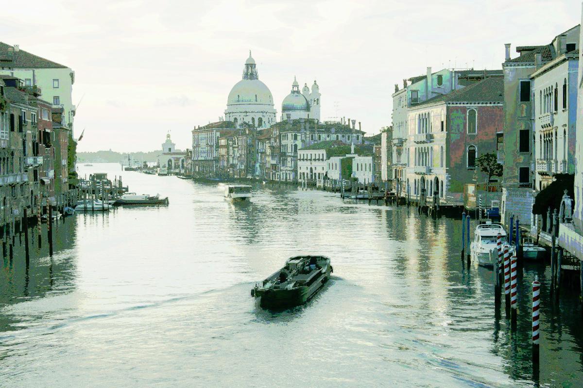
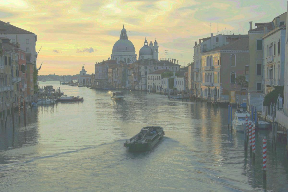
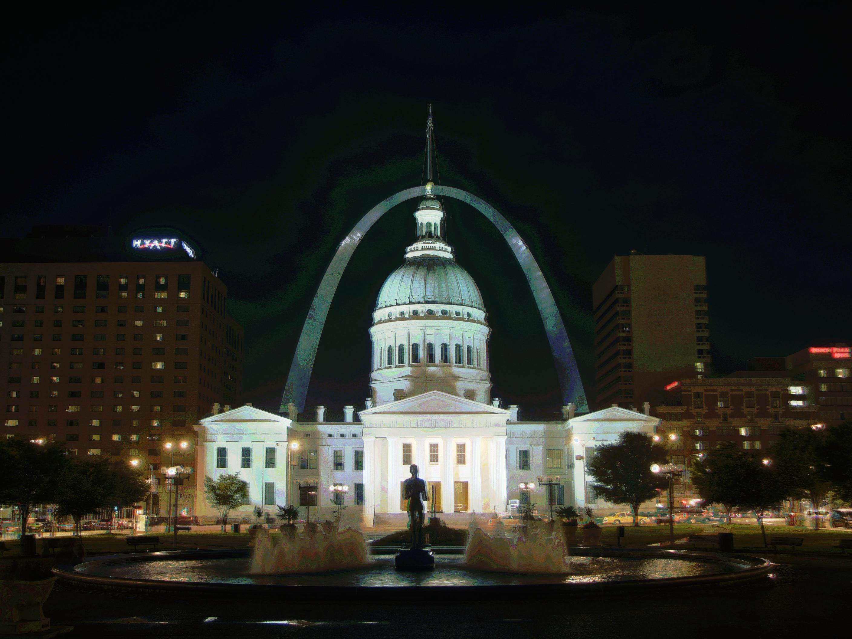
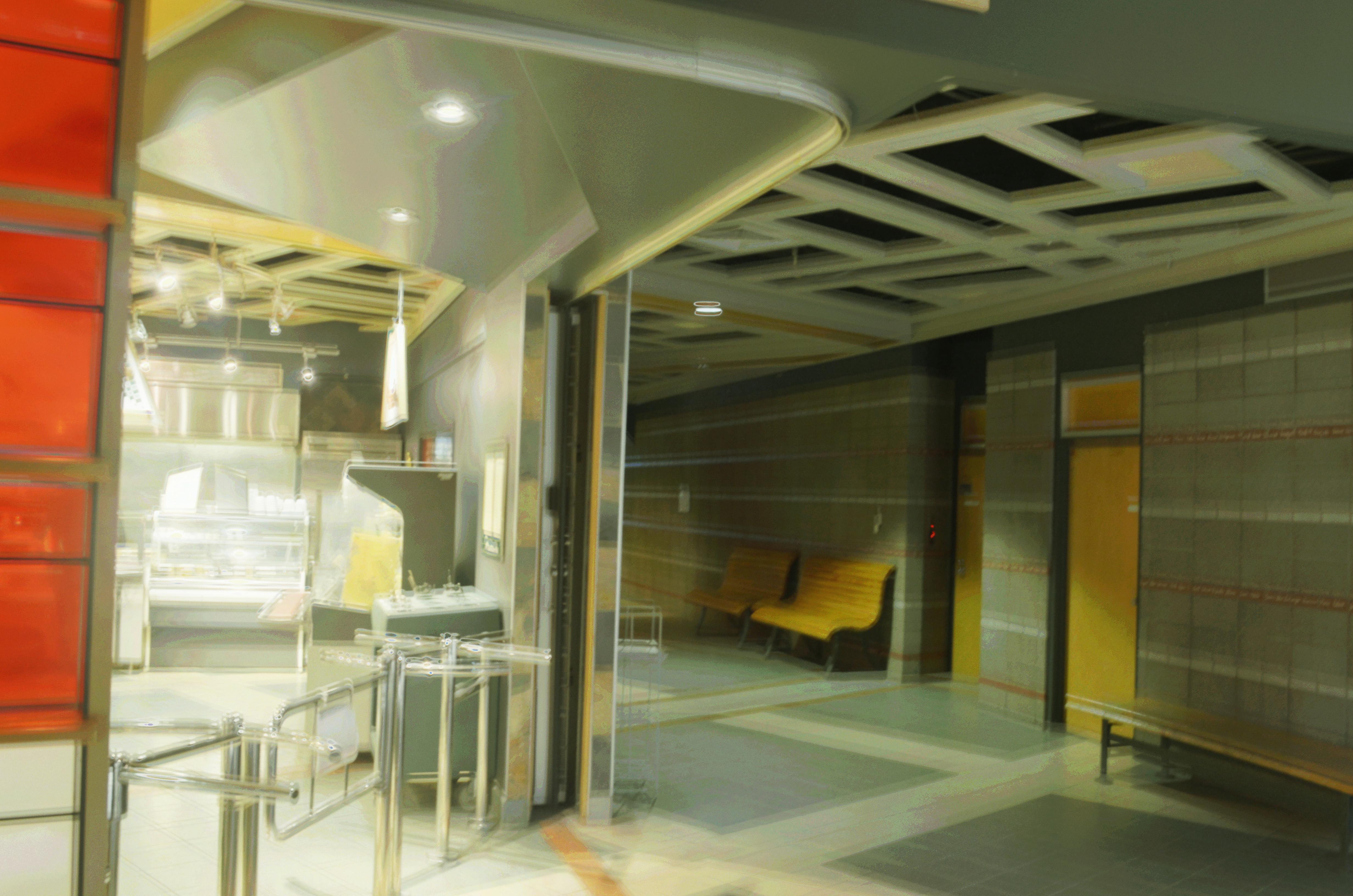
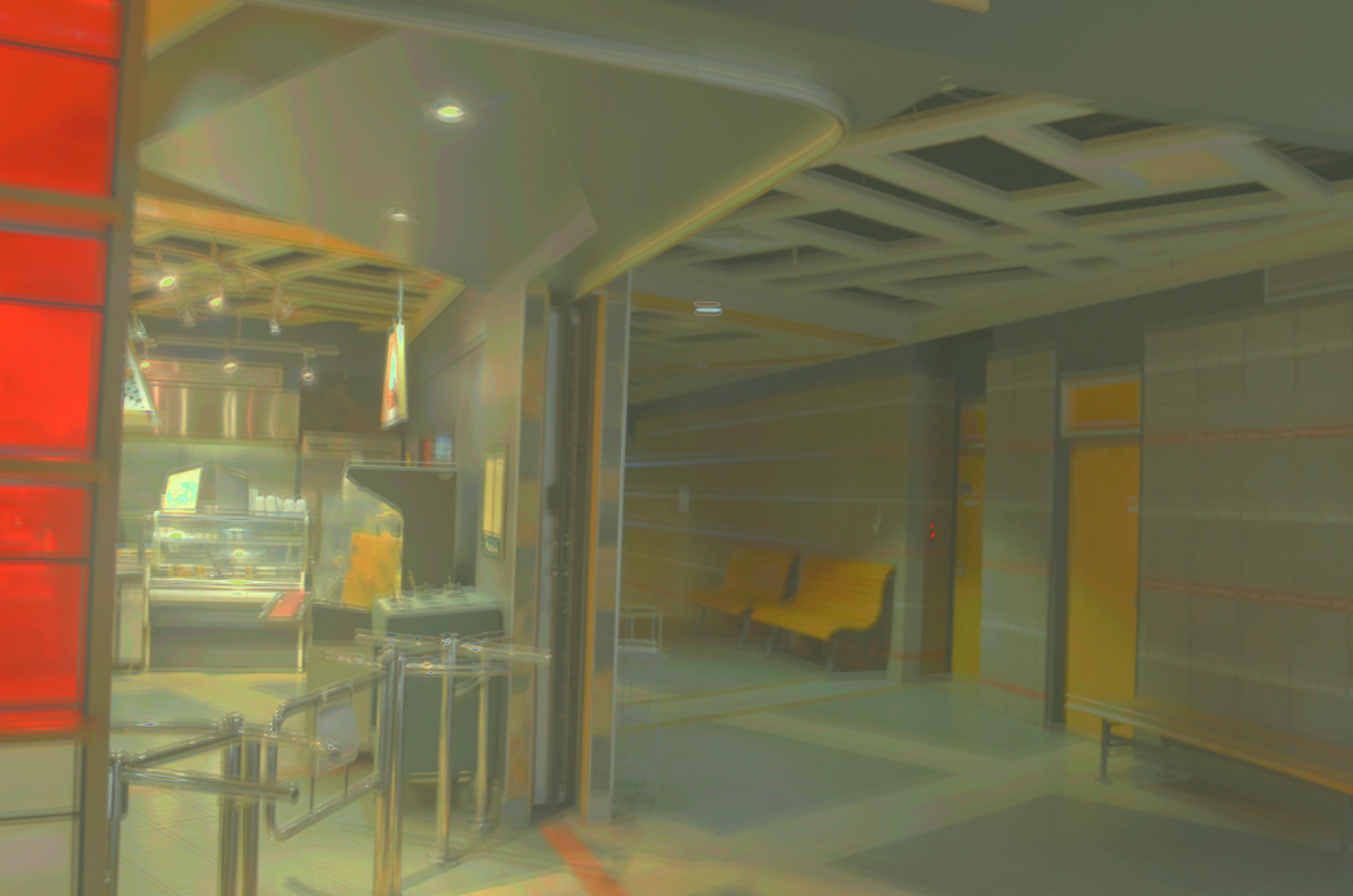
Experimental Results for Tone Mapping

Global	Local

Global	Local

Global	Local

Global	Local

Bells and Whistles

Use My Own Images

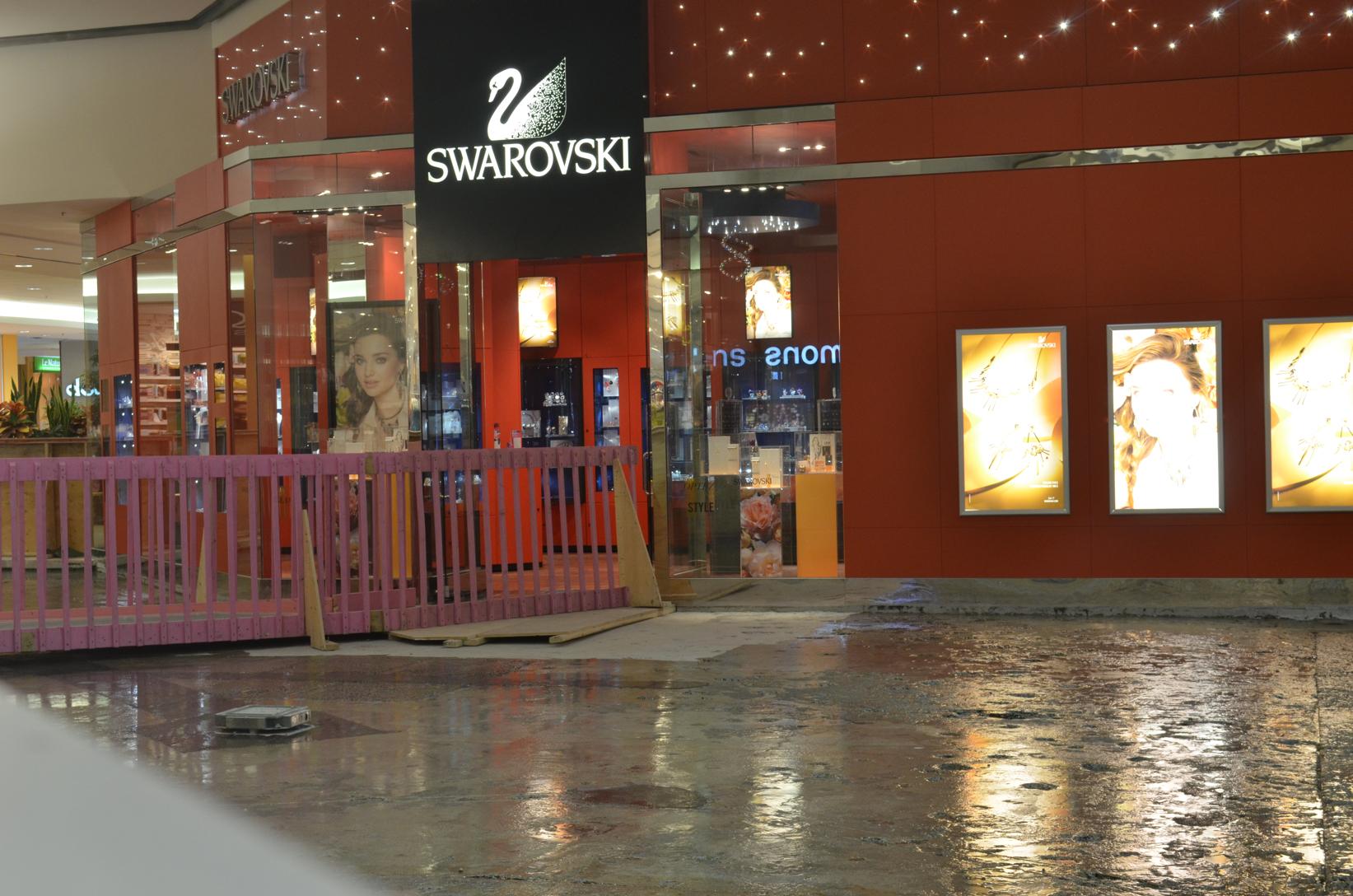
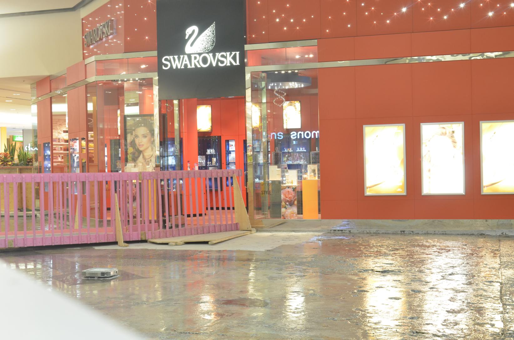
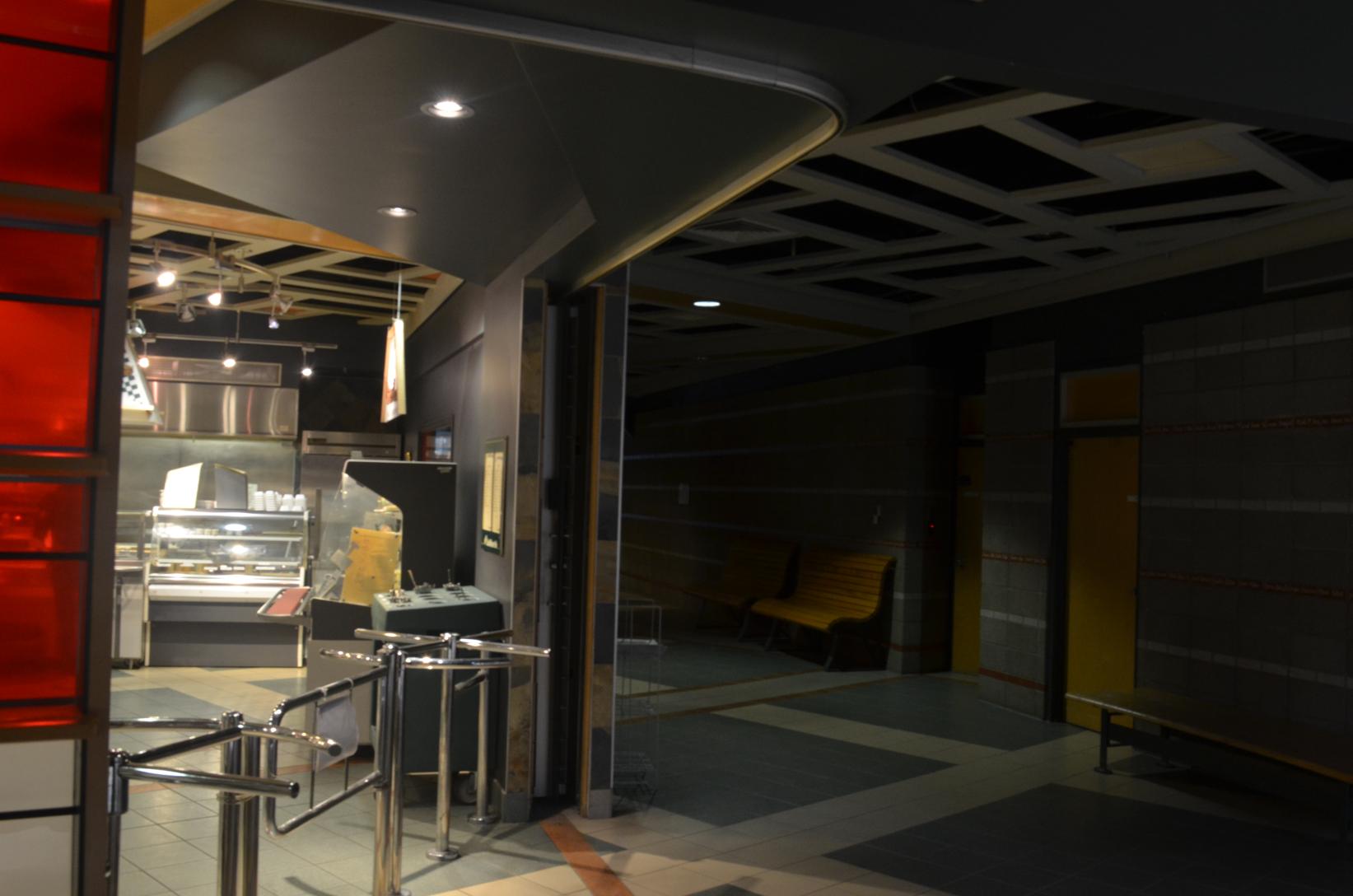
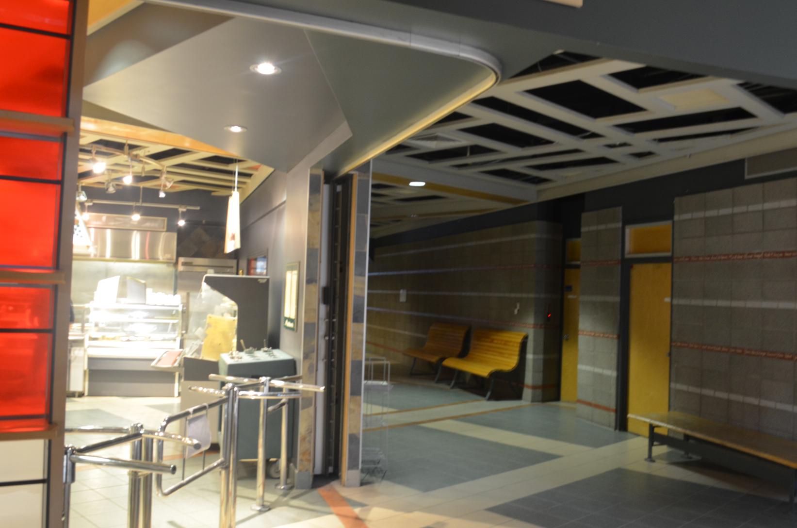
For this project, I have taken some photos from differen places.

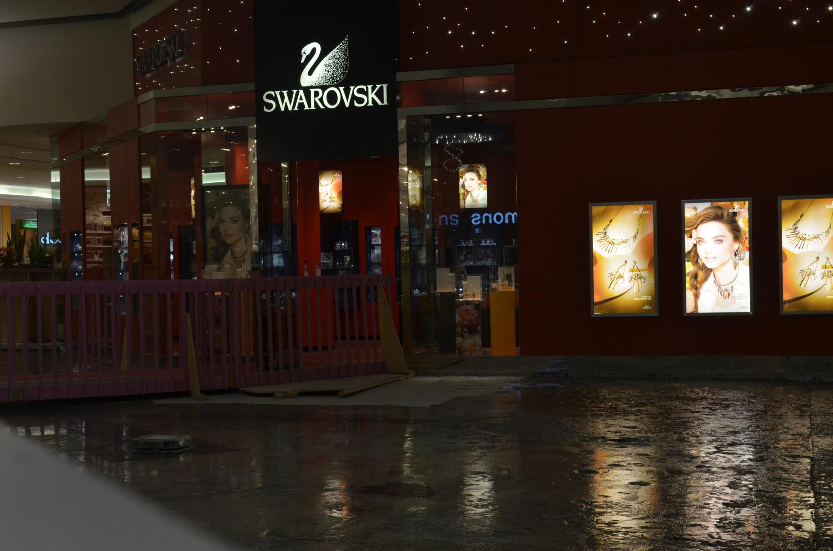
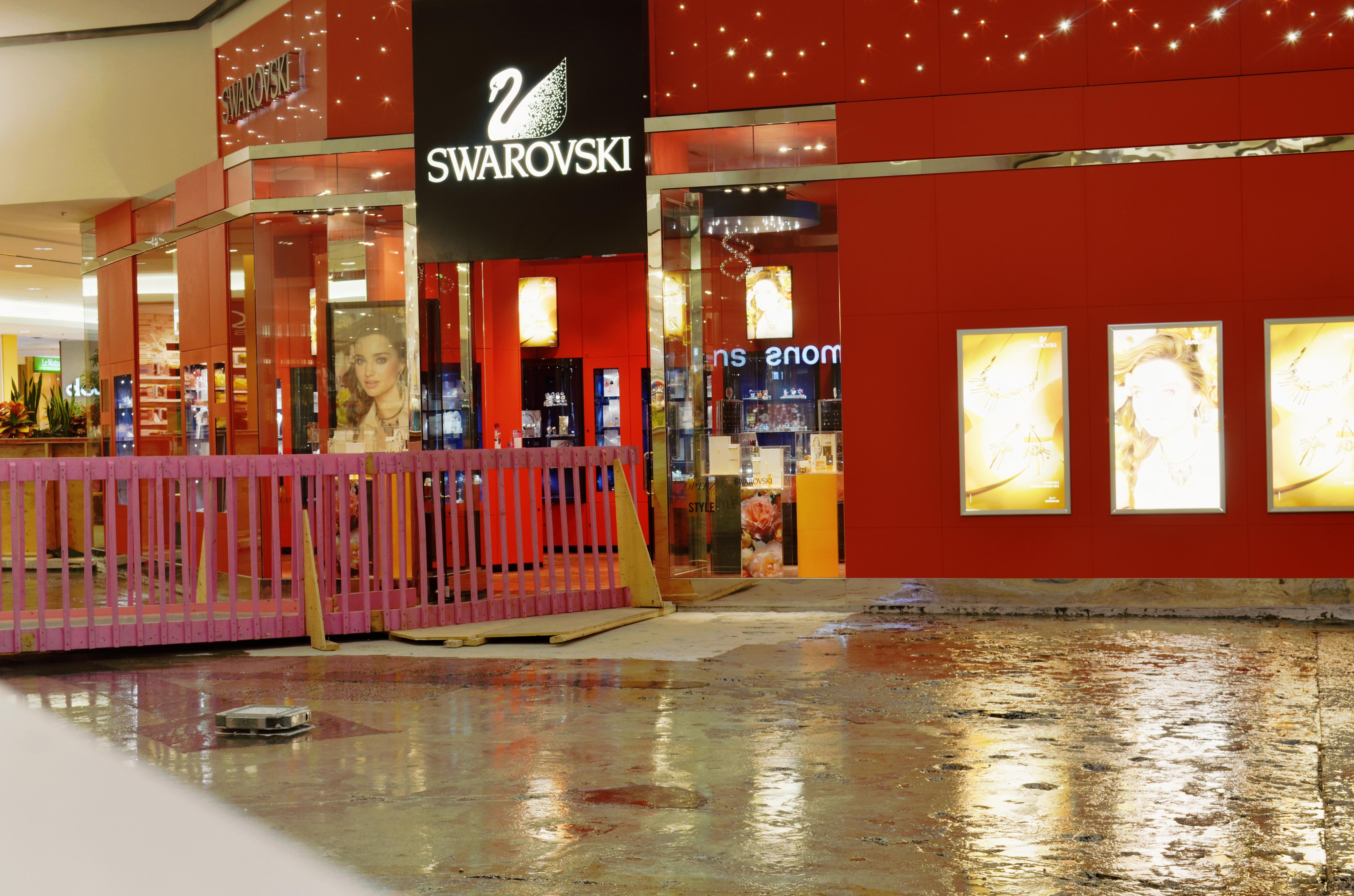
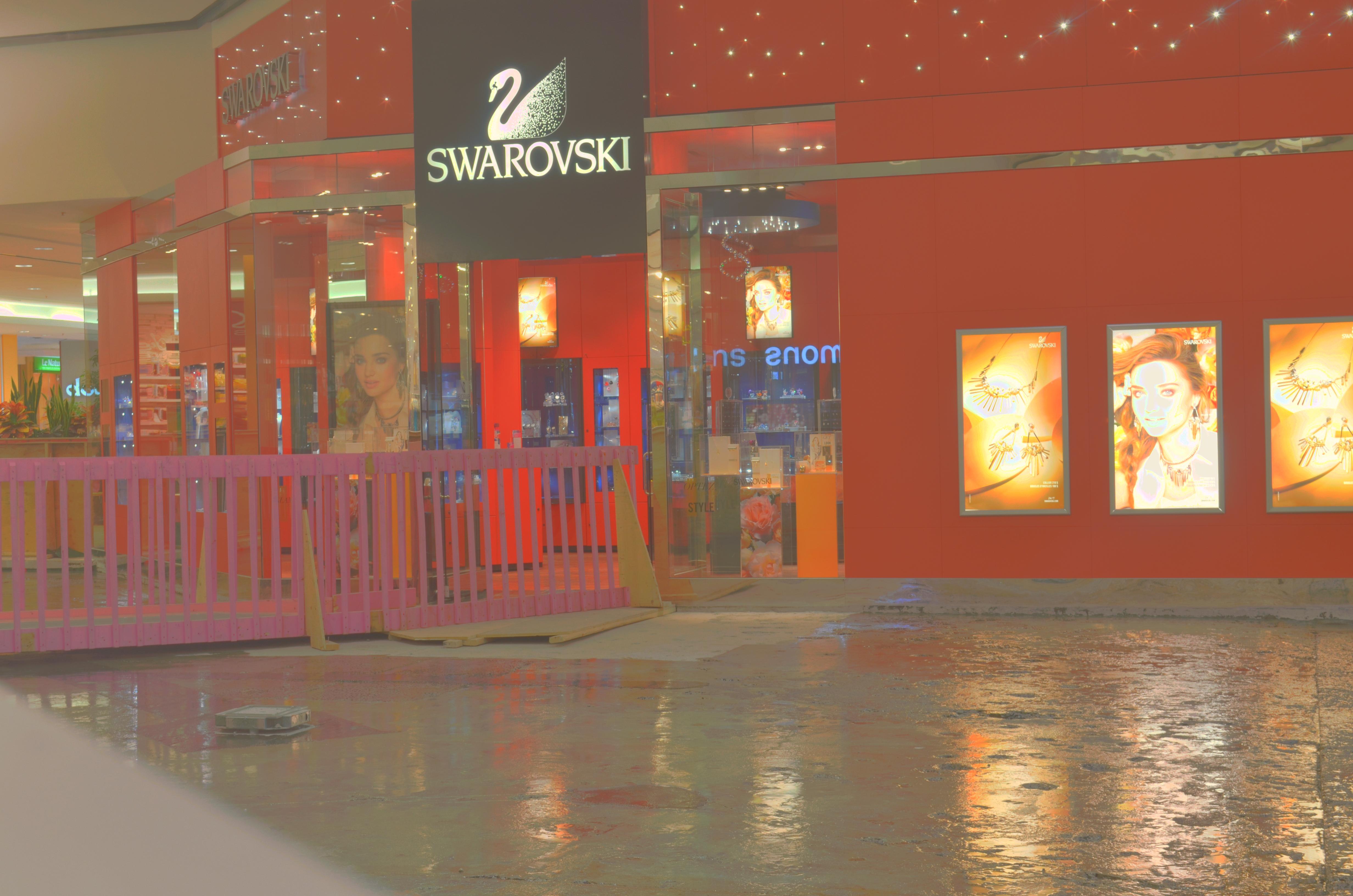
Photos from Swarovski Store

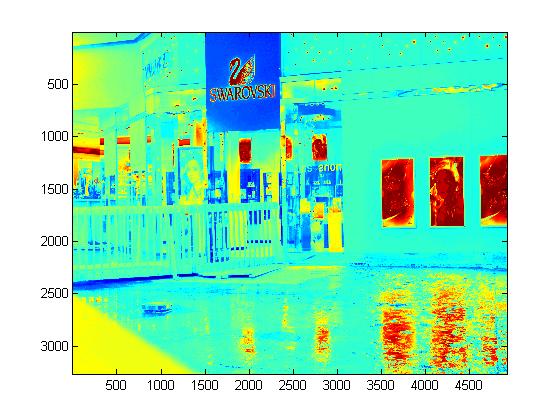
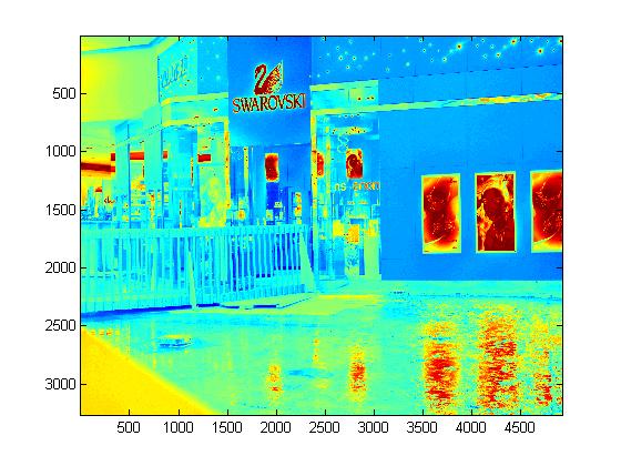
Experimental Results

Global	Local

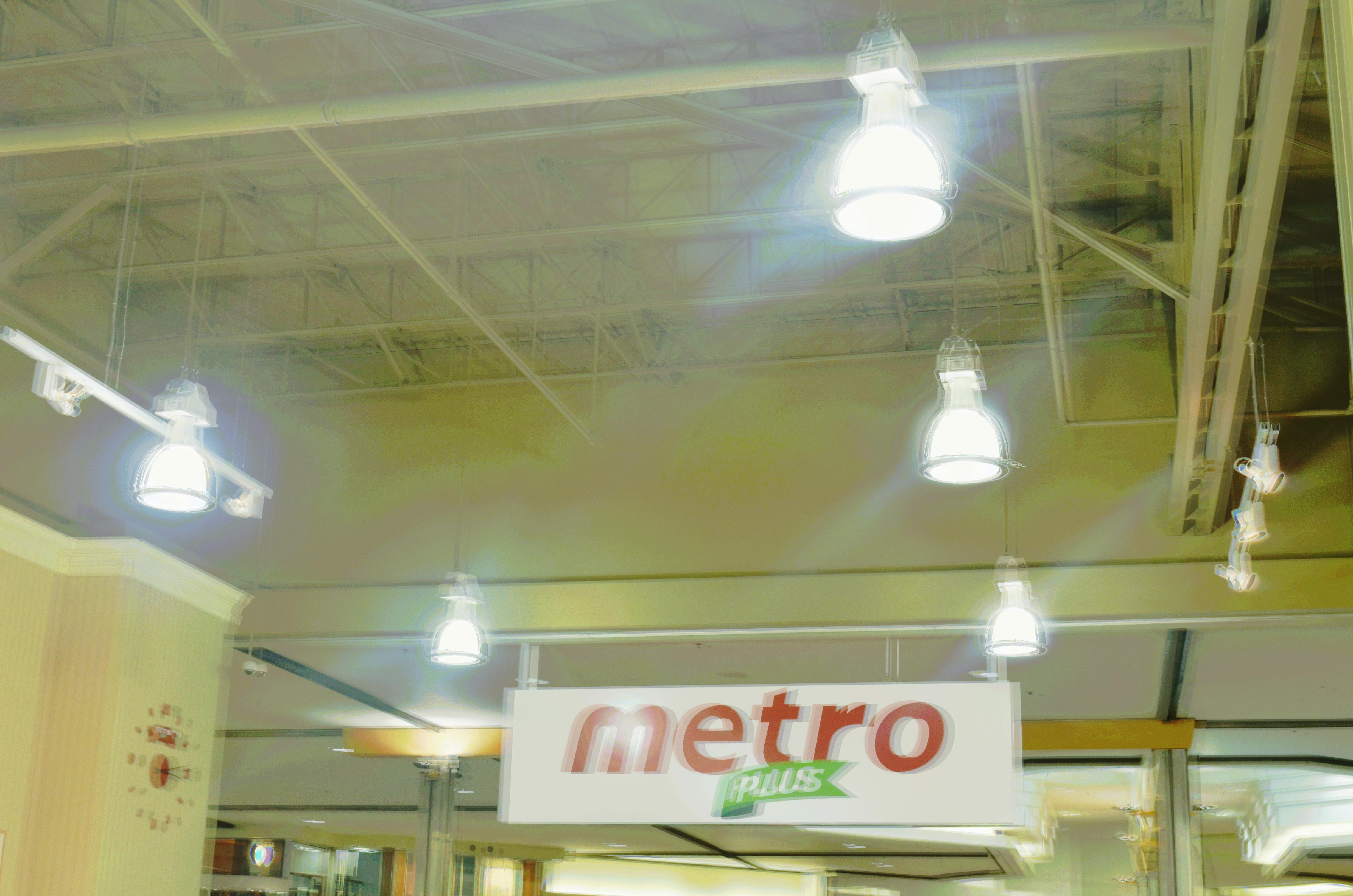
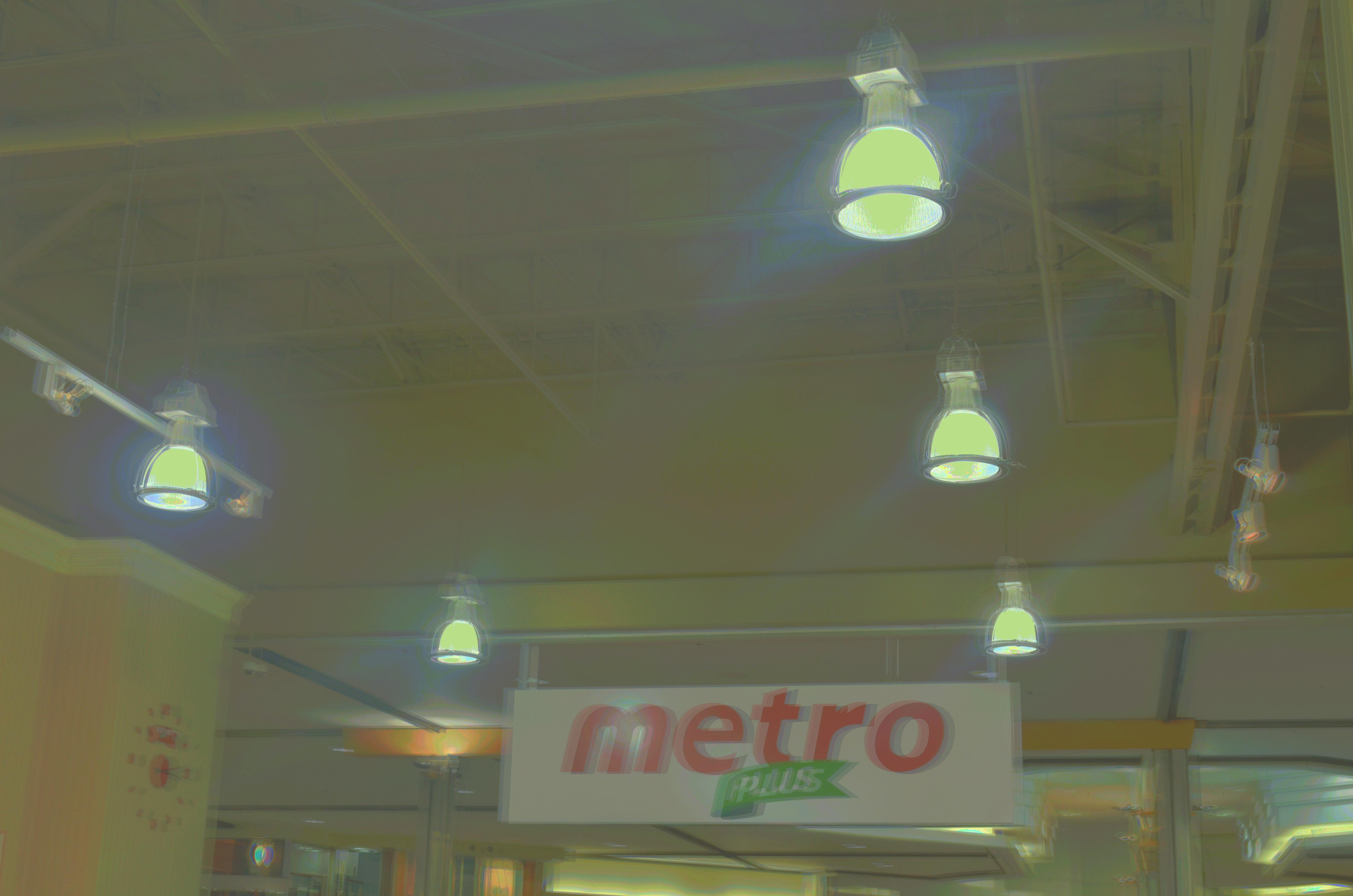
Photos from Metro Supermarket

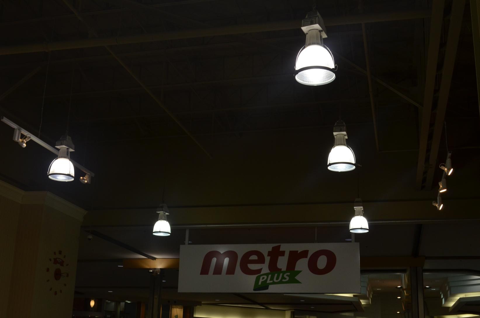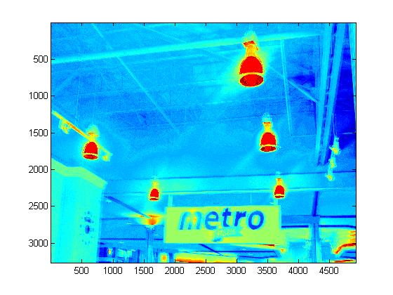
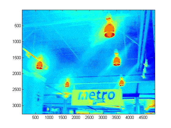
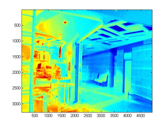
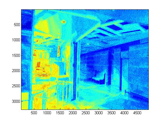
Experimental Results

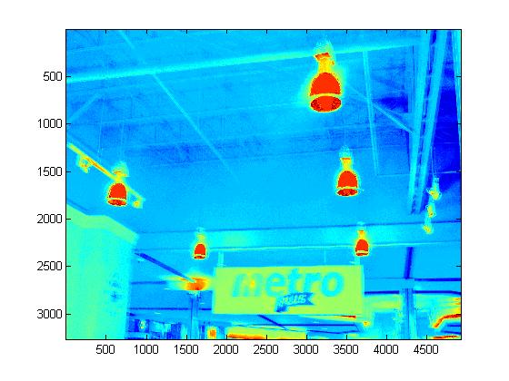Global	Local

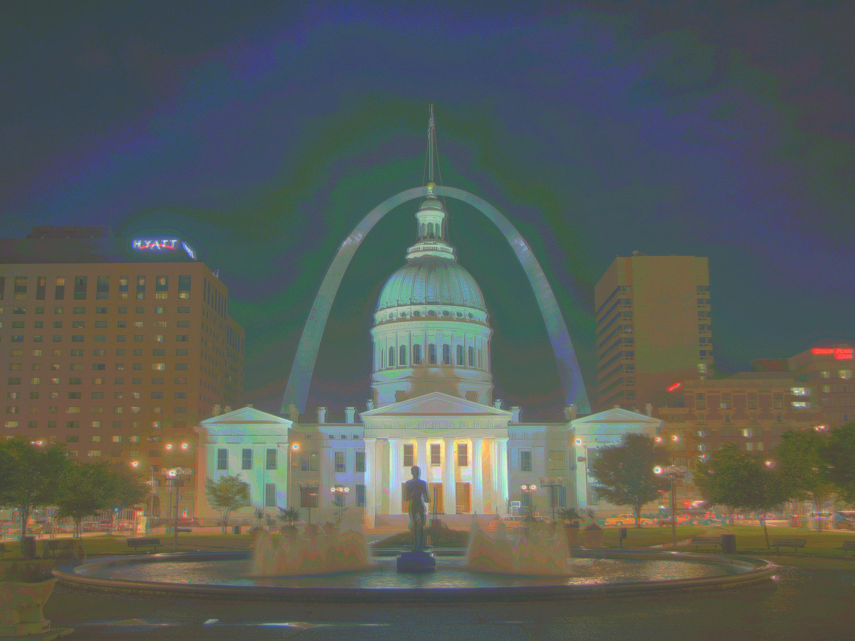
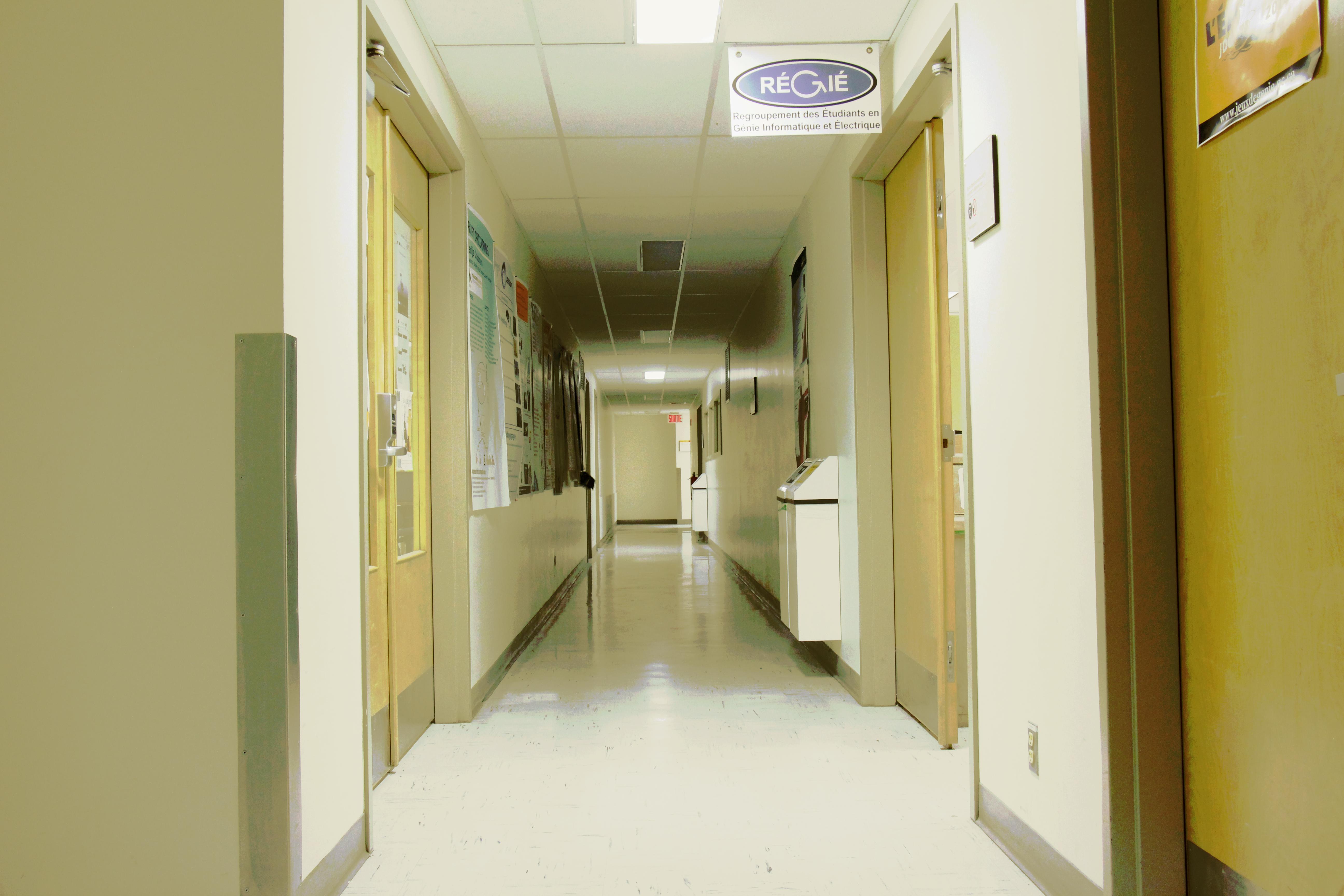
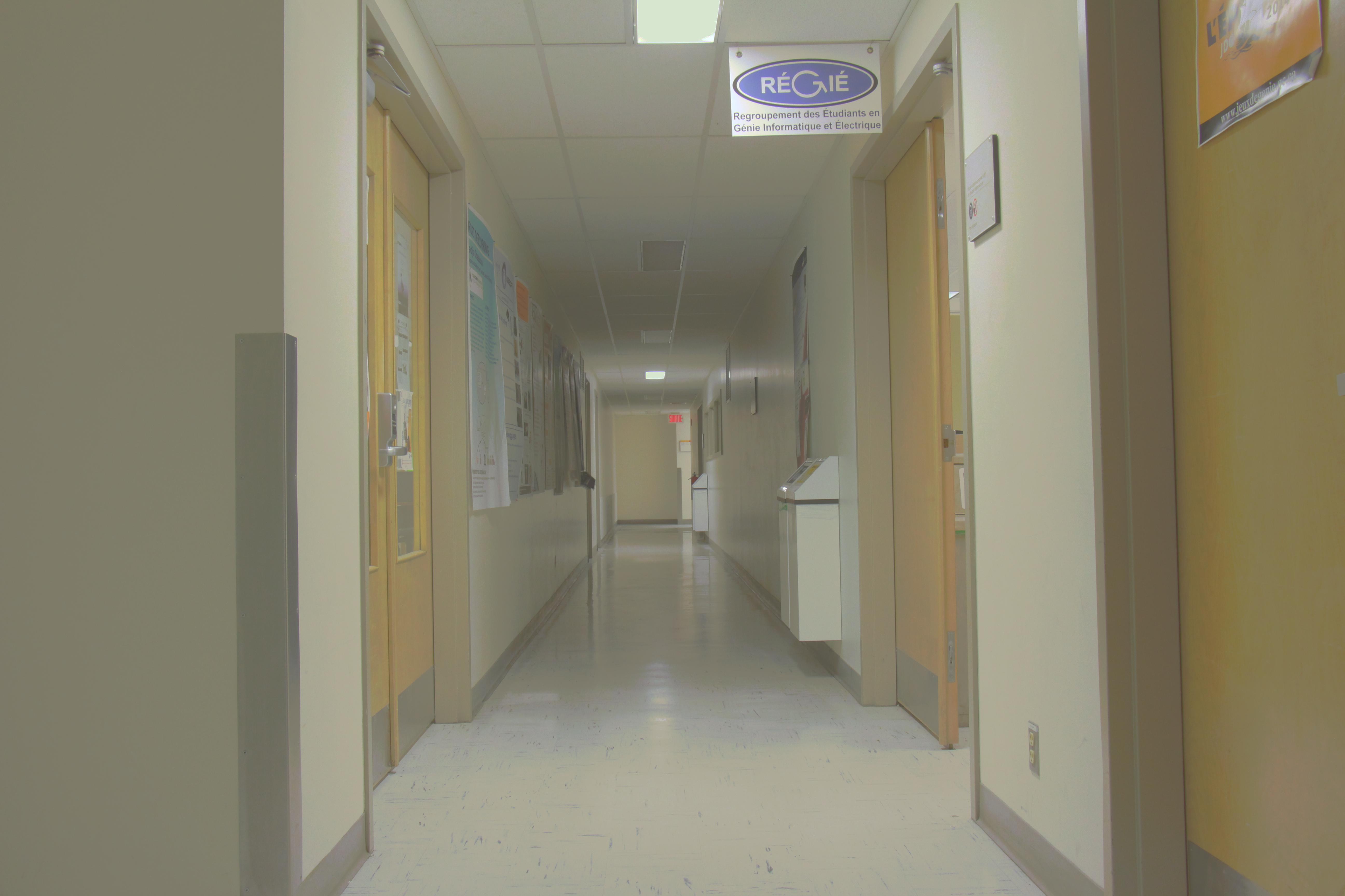
Photos from Pavillon Desjardin

Experimental Results

Global	Local

Optimized Bilateral Filtering

For the optimized bilateral filtering, I choose the fast bilateral filter. As the direct implementation of bilateral filter includes two nested loops, its computational complexity is \(O(s^2)\) where s is the number of pixels. So for some high-resolution image, the brute-force version of bilateral filter will be extremely slow. The fast bilateral filter is proposed by Durand and Dorsey based on the observation that this filter is almost a convolution of the spatial weight \(f(p-s)\) with the product \(g(I_p-I_s)I_p\). If the latter product is independent on the intensity of each pixel \(I_s\), it will turn to be a complete convolution. So the speed challenge is overcome by picking a fixed set of sampled intensities \({I_1,I_2,...,I_n}\). So we can get a set of \(J_i,i=1,...,n\). For the intensities that have not been sampled, I compute the result using linear interpolation between two \(J_i\) who has the closest intensity values. And this method further accelerate the computation by down-sampling the image as first. The final \({I_1,I_2,...,I_n}\) is obtained by up-sampling the convolution outputs. The bilateral filtering results are still obtained by linearly interpolation.

Gradient Domain HDR Compression

As is inspired by professor's suggestion, I implement a simplified version of the gradient domain compression for the display of HDR image on LDR devices. This is really a non-trivial task for me. It mainly contains two steps. The first step is to get the gradient field of the HDR radiance map and do some manipulation to the gradient field. To compress the gradient of each pixel, we add a factor \(\psi(x,y)\) to each corresponding gradient of each pixel. As is suggested in the paper, we set the factor \(\Psi(x,y)\) as following: \[\psi(x,y)=\frac{\alpha}{||\bigtriangledown H_k(x,y)||}(\frac{||\bigtriangledown H_k(x,y)||}{\alpha})^{\beta}\] \(\alpha\) determines which gradient magnitude will remain unchanged. Gradient magnitude which is larger than \(\alpha\) will be attenuated while the smaller one will be enlarged. We set \(\alpha\) to be the average gradient magnitude multiplied by 0.1 and \(beta\) to be 0.85.

After we get the attenuated gradient field, we need to reconstruct the new HDR radiance map from this new gradient field. This task can not be accomplished by simple integration as for the 1-D case. As is illustrated in the paper, we need to minimize the integral: \[\int\int F(\bigtriangledown I,G)dxdy\]. And according to the Variational Principle, it must satisfy the Euler-Lagrange equation: \[\frac{\partial F}{\partial I}-\frac{d}{dx}\frac{\partial F}{\partial I_x}-\frac{d}{dy}\frac{\partial F}{\partial I_y}\]=0 After some derivation, we get the Poission equation \[\bigtriangledown^2I=divG=u(x,y)\] I solve this famous equation using linear approximation. This will produce a linear system. But instead of using Full Multigrid algorithm to solve the linear equation system, I use Discrete Sine Transform to solve the linear system. The process can be illustrated as following steps:
(1)Compute 2D sine transform of \(u(x,y)\)
(2) Divide by eigen values
(3) Compute 2D inverse sine transform
(4)\(I(x,y)=idst2(\frac{dst2(u(x,y))}{\lambda(x,y)})\)

After we get the new compressed radiance map, I assign the R G B colors to each corresponding pixel as follows:\[C_{out}=(\frac{C_{in}}{L_{in}})^sL_{out}\] where \(C=R,G,B\). \(L_{in}\) and \(L_{out}\) represents the luminance before and after HDR compression.

Gradients of the HDR radiance map	After gradients attentuation