Feature Matching

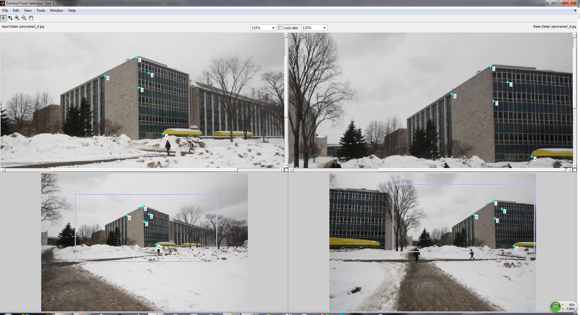
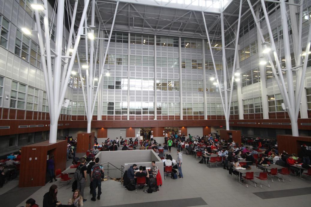
For feature matching, I use the "cpselect()" function to select the corresponding points between to images. After that, I use the "cpcorr()" function to modify and refine the position of the points. To compute a homography, at least 4 pairs of corresponding points is needed. The process of estalishing correpondence should be done with carefulness. As is illustrated in the figure, I usually choose the point which located at the corner of an object. The gradient of those locations are always larger than oher points.

Compute Homography

After establishing the correspondence between two images, the homography matrix is to be computed from those corresponding points. The homography matrix is needed to compute the warped image so as to align them. The homography matrix contains the parameters of transformation between each pair of images. The homography matrix \(H\) is denoted as follows:

\[ \left[\matrix{wx_i' \cr wy_i'\cr w\cr}\right]=\left[\matrix{H_{11} & H_{12} &H_{13}\cr H_{21} & H_{22} & H_{23}\cr H_{31} & H_{32} & H_{33}\cr}\right]\left[\matrix{x_i \cr y_i\cr 1\cr}\right] \]

Warping

After knowing the parameters of the homography matrix, I need to warp all the target images to the plane of the base image. Before warping, we need compute all the homography matrix and get the largest bounding box so as to make it can contain all the warped image in a uniform coordinate system.

Image blending

Now we have all the mosaic images which has been mapped to a uniform coordinate system. We can compose them simply by "max()" function, because for the overlapped part we just need to display the max R G B intensity value of the warped image one by one. The results shows that this approach can achieve our goal of image stitching.

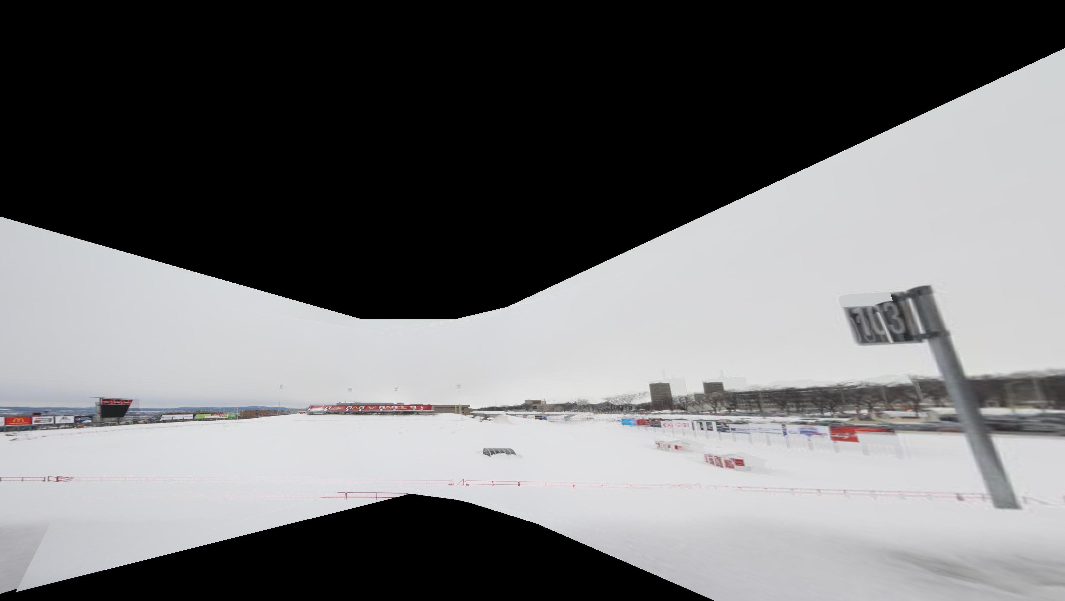
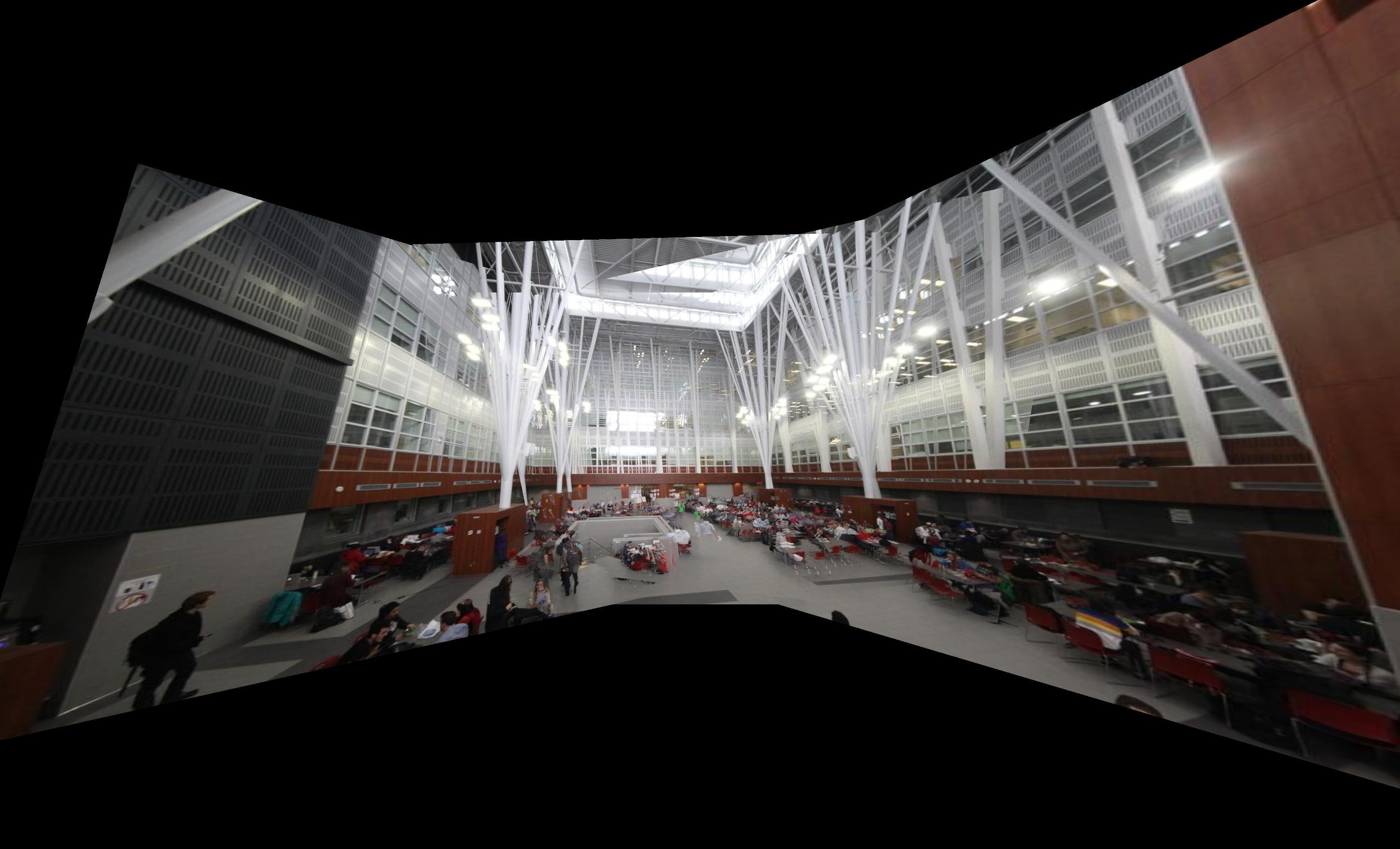
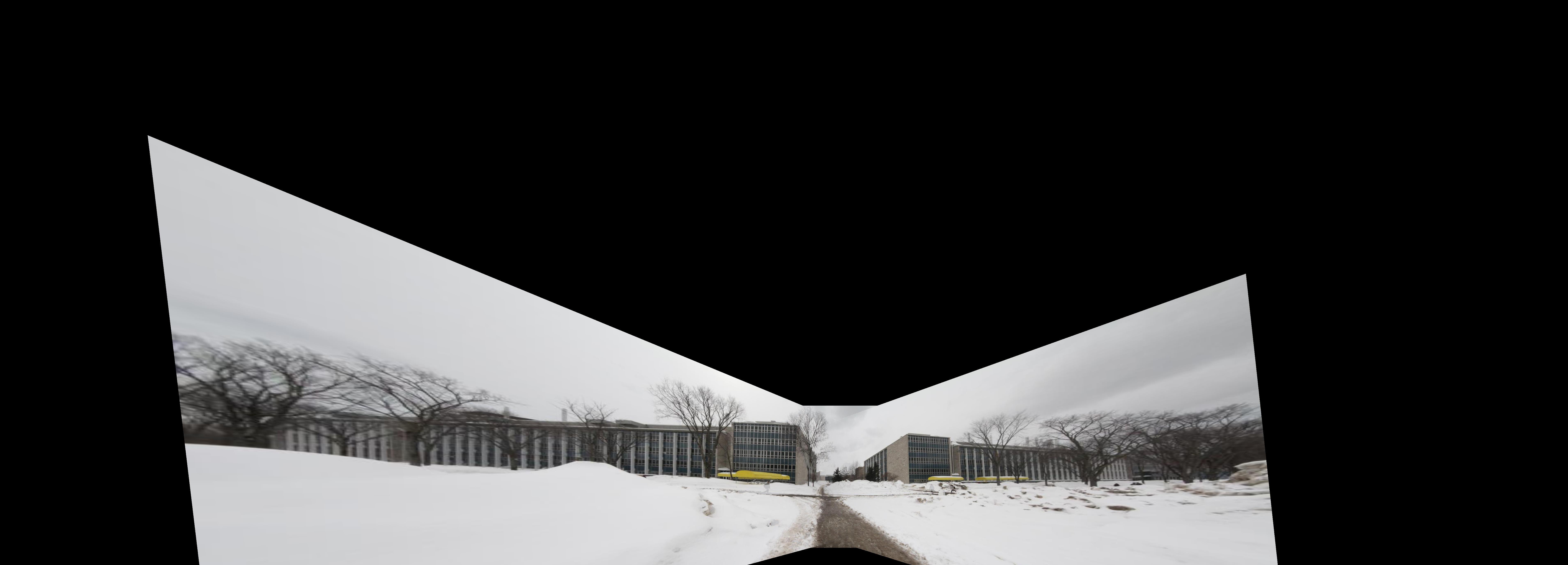
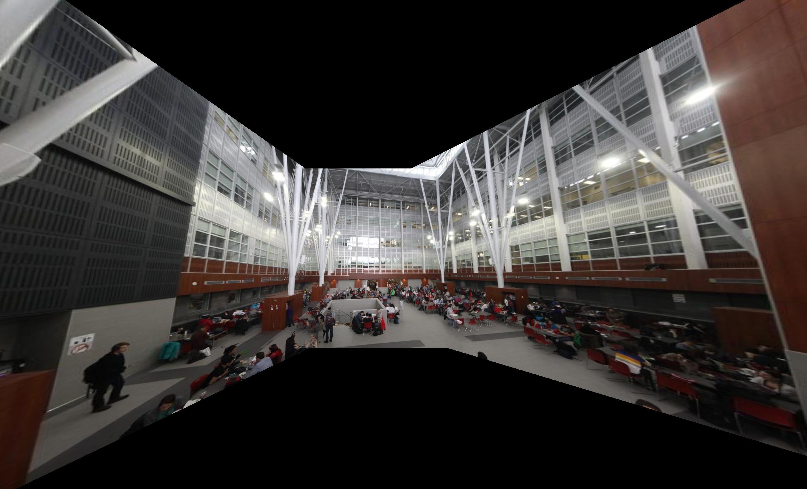
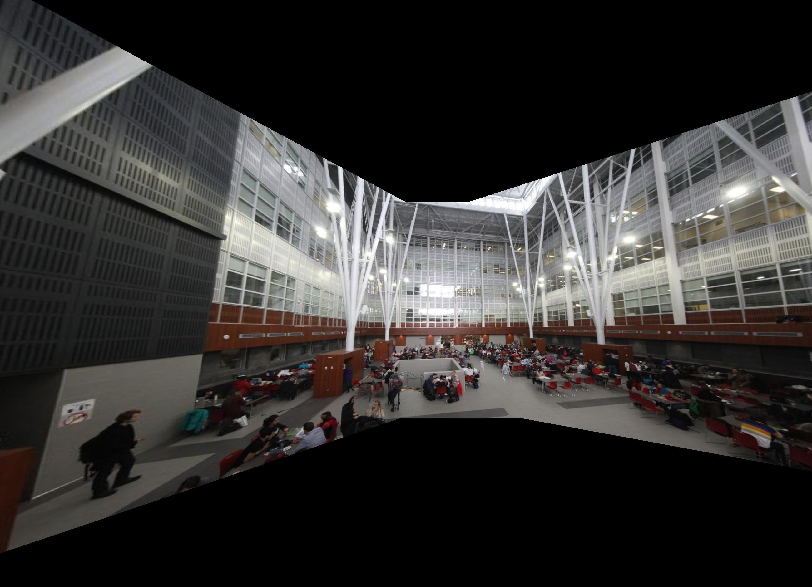
Experimental Results for Manual Matching

Part 2: Automatic Matching

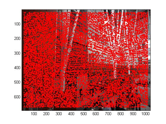
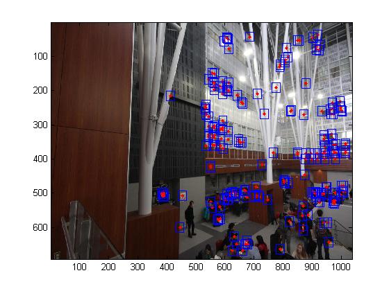
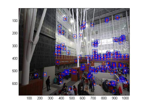
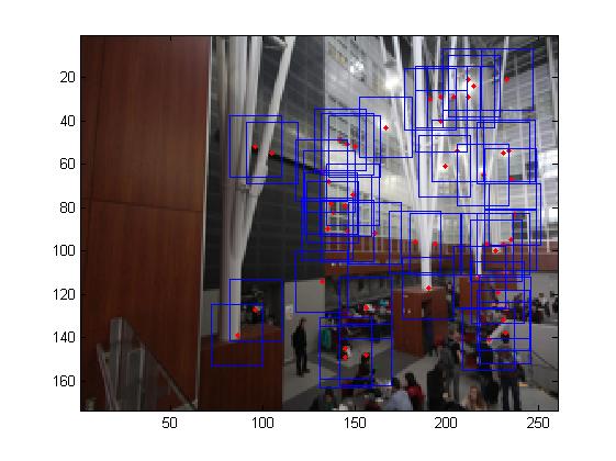
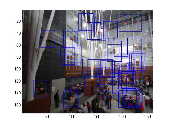
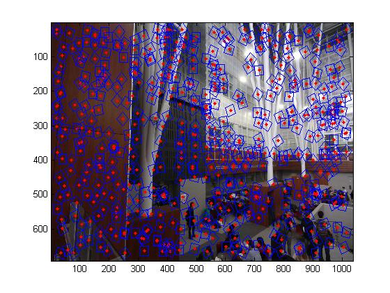
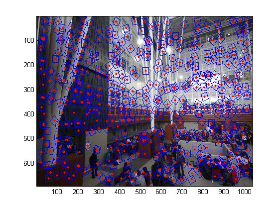
Detecting corner features in an image

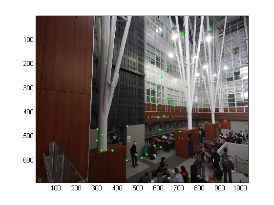
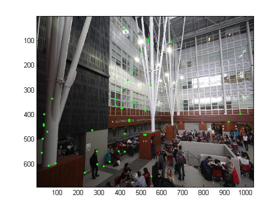
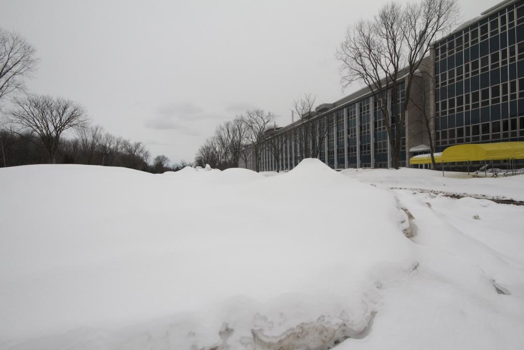
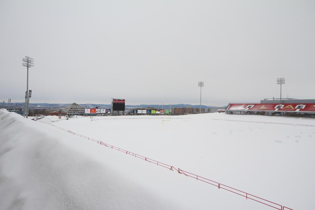
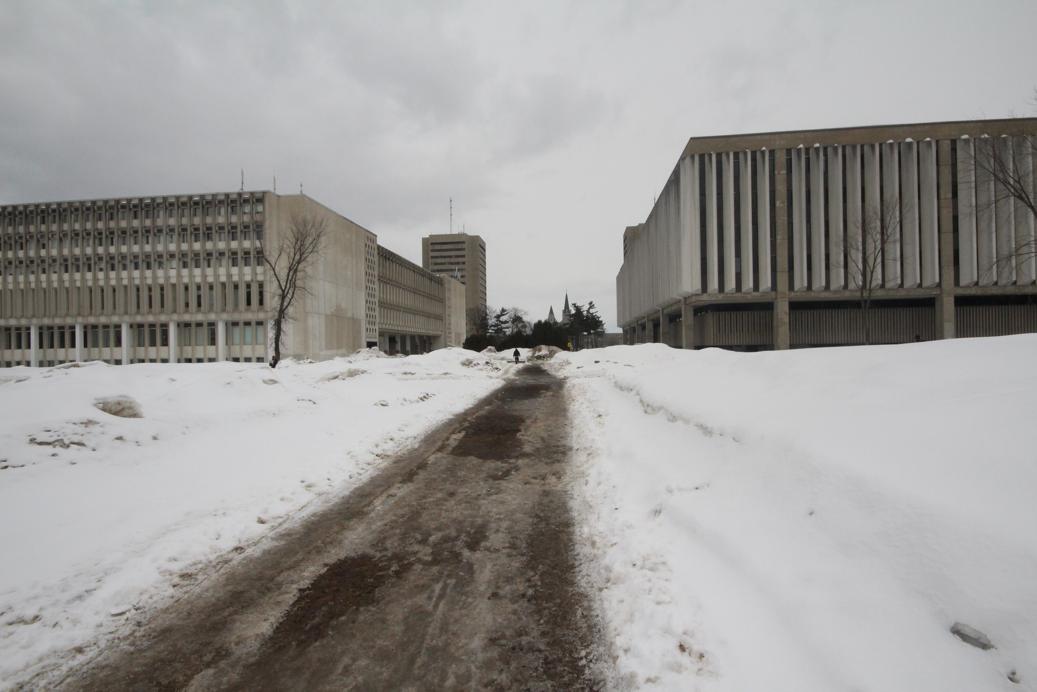
To do the automatic image matching, first we need to detect the image keypoints. The first step is to search the Harris corner feature. A Harris corner feature in an image is a location where the horizonal and vertical gradients are both very strong.But we need to notice for some pictures we has some uniform color area such as the field covered with snow, the corner feature that we detected do not have high value and those bad feature will devastate the results. So we need set up a threshold for the image feature value or sort them in descending order and select the top N.

\[A=G*\left[\matrix{I_x^2 & I_xI_y\cr I_xI_y &I_y^2}\right]\]

where \(I_x\) and \(I_y\) are the image intensity derivatives, and\(G\) is a Gaussian kernel, the Harmonic mean score \(f_{HM}\) is defined as

\[ f_{HM}=\frac{Det(A)}{Trace(A)}\]

A point \( (x,y) \) in the image is a corner if \(f_{HM}(x,y)>threshold\).

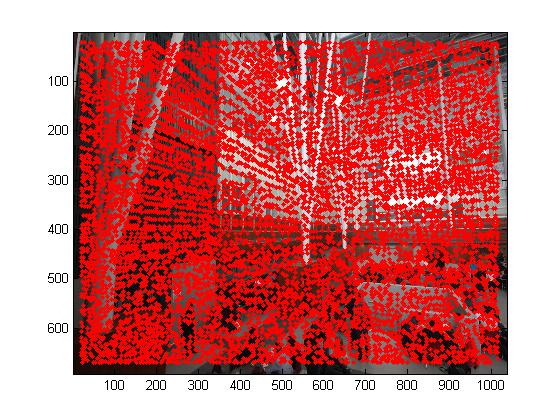
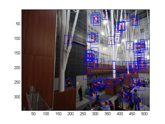
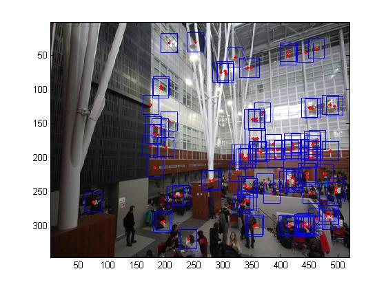
The second step is to use the adaptive non-maximal suppression which is mentioned in the paper to filter the features. ANMS is used to select a subset of all the keypoints which have high corner score and which averagely spatially distributed in the image. ANMS is easy to implement. Loop through all the initial keypoints, and for each keypoints compare the corner strength to all other keypoints. Keep track of the minimum distance to a larger magnitude keypoint. \(r_i=min_j|x_i-x_j| s.t. f_{HM}(x_i)<0.9f_{HM}(x_j)\) After you have computed this minimum radius for each keypoint, sort the list of keypoint by descending order and take the top N.

Extracting a feature descriptor for each feature point

In my implementation, the descriptors are sampled from a larger 40*40 square patch centered at the keypoint location. Each descriptor is represented as a 8*8 normalized matrix. Normalization is done by substracting to each entry the mean value and dividing it by the standard deviation.

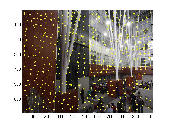
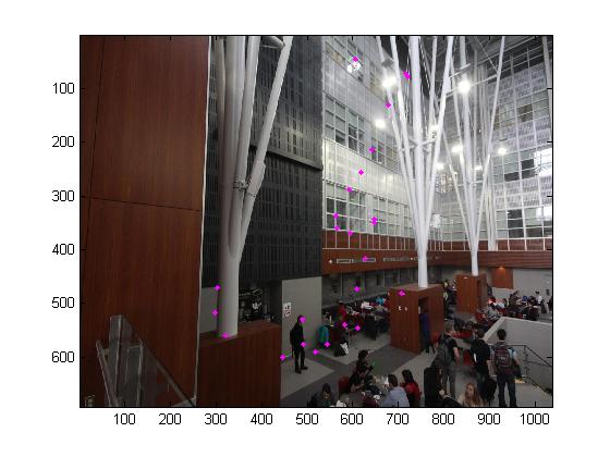
Matching these feature descriptors between two images

To find pairs of matched features, we use the Euclidean distance to find the nearest and second nearest neighbors of each descriptor. We take the Lowe's simple method on thresholding the ratio between them. In my experiment, the threshold is 0.5.

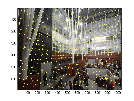
Using RANSAC (Random Sample Consensus to compute a homography)

After feature space outlier rejection, there are still too many outliers. So we use a RANSAC(Random Sample Consensus) for rejecting the outliers progressively. The algorithm of RANSAC for estimating homography is recursive. Each loop contains four main steps. First, four feature pairs is selected randomly. Second, compute the homography matrix using the four selected points. Third, compute inliers \(||p_i',Hp_i'||<\epsilon\) At last, keep the largest set of inliers. And once we get the largest set of inliers, the homography matrix is recomputed by least-square method.

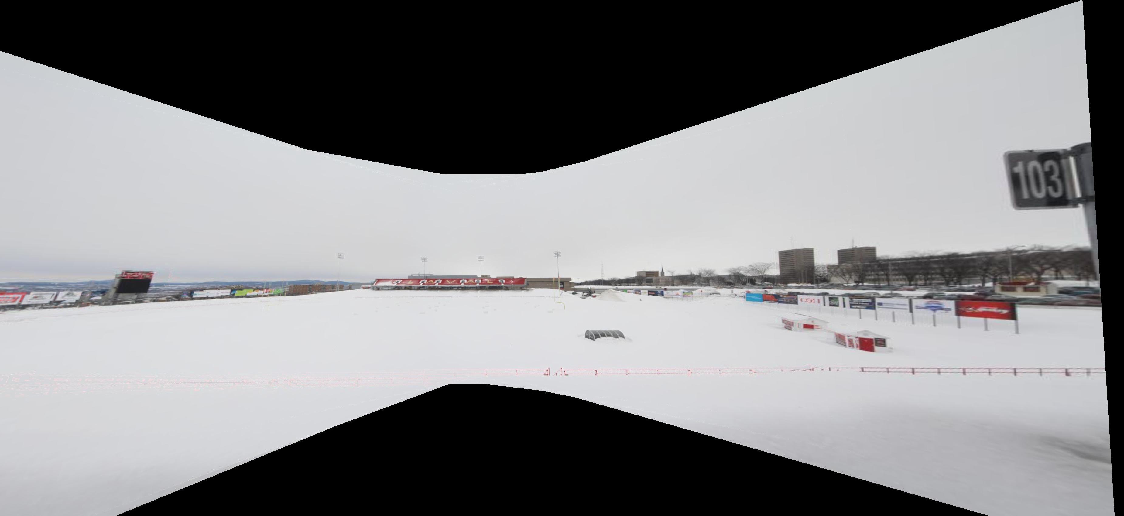
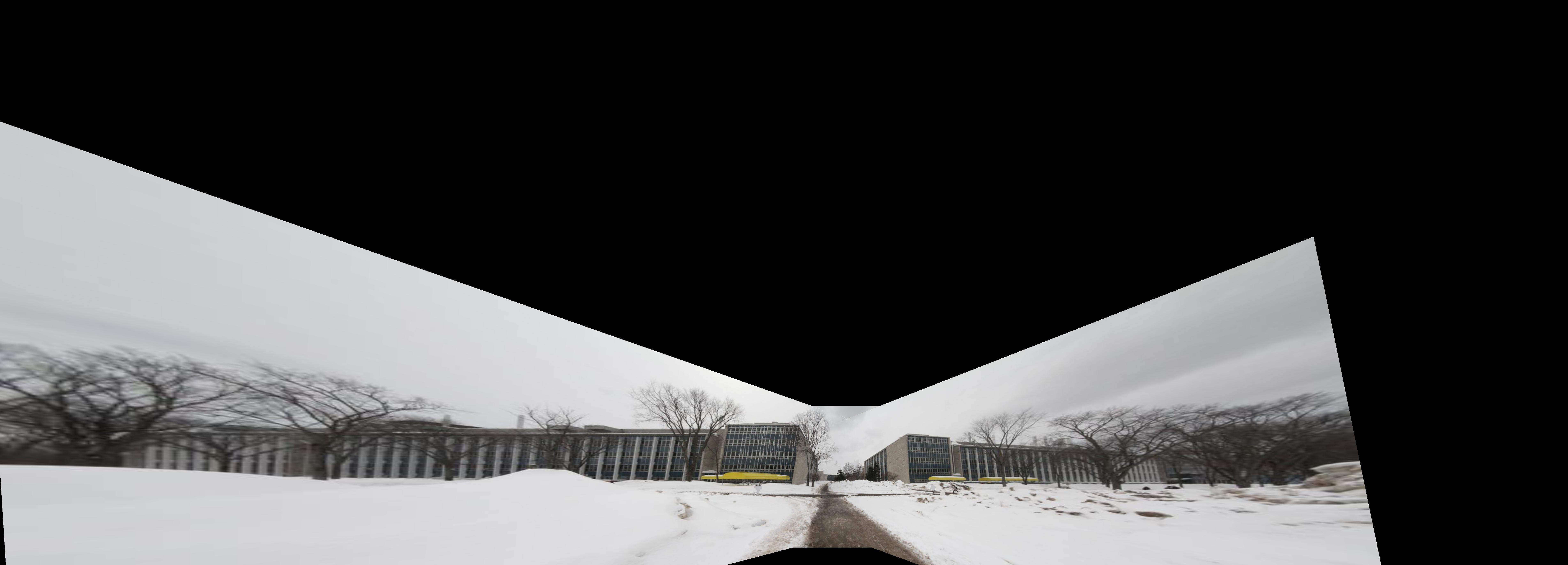
Experimental Results for Automatic Matching

Bells and Whistles

Blending and Compositing

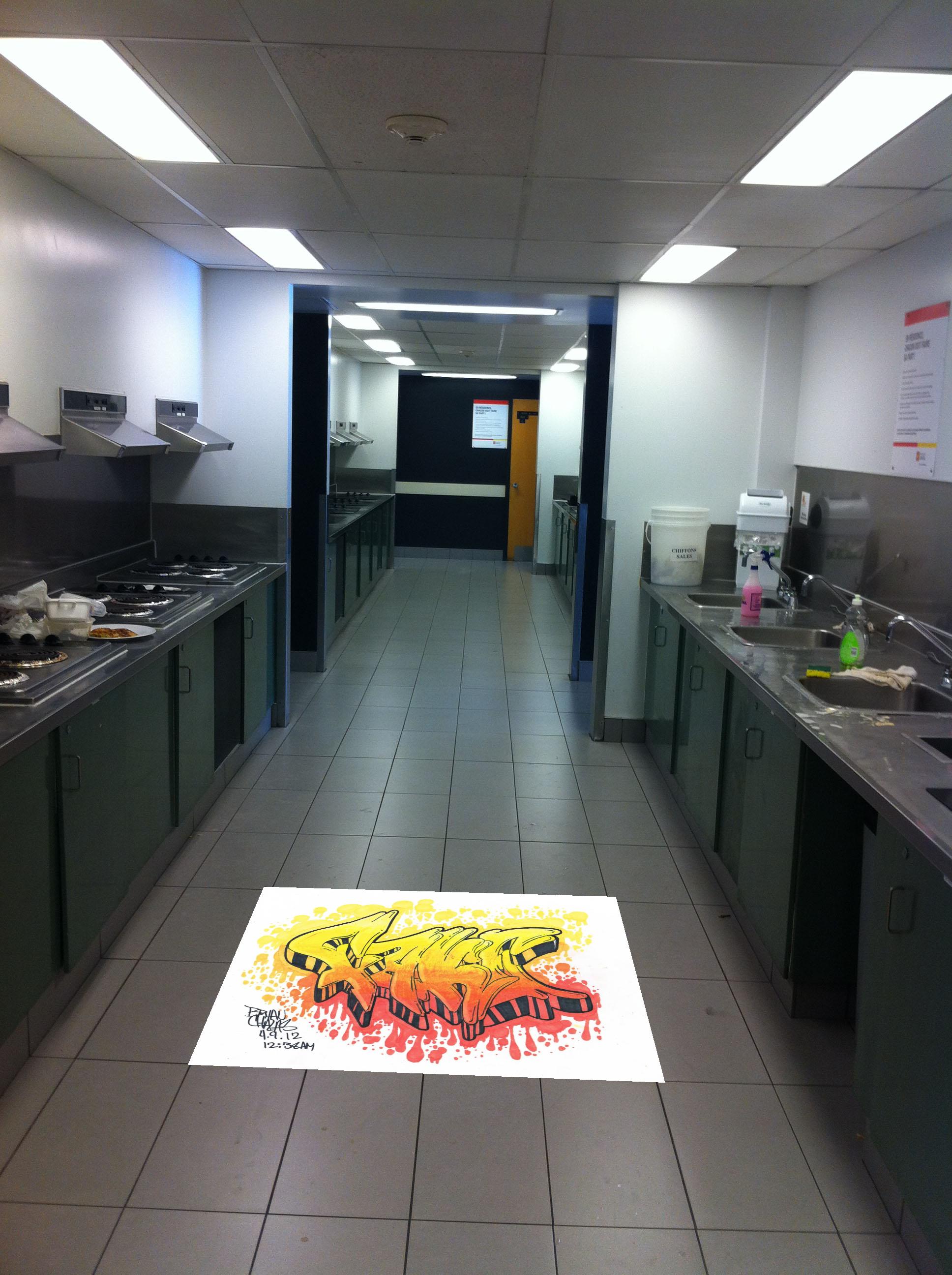
Fake graffiti

I took the graffiti image from internet and used the image in my camera taken from kitchen in Pavillon Parent.

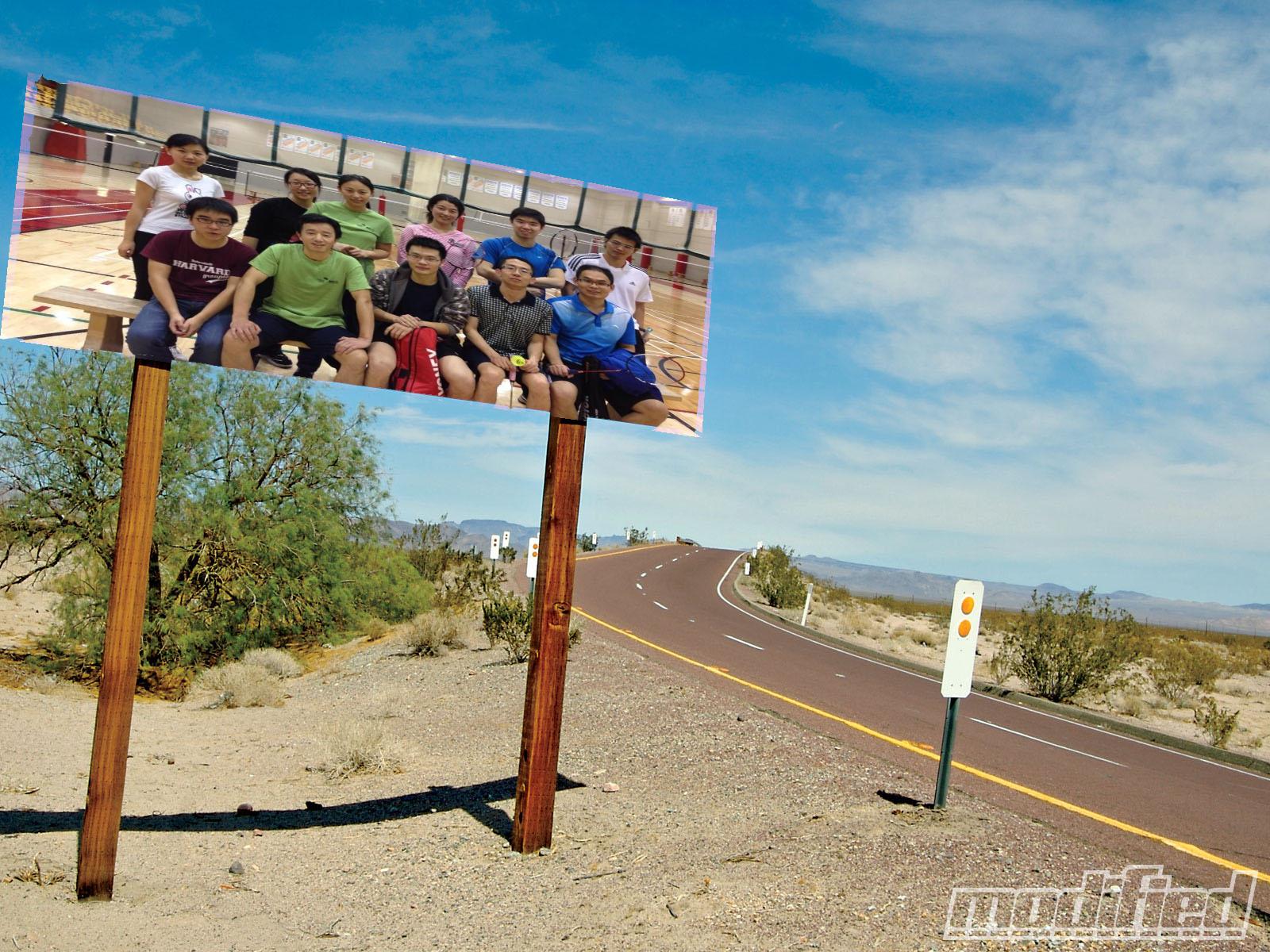
Fake road sign

I took the road sign image from internet and used the image in my camera taken from peps when I was playing badminton with my friends.

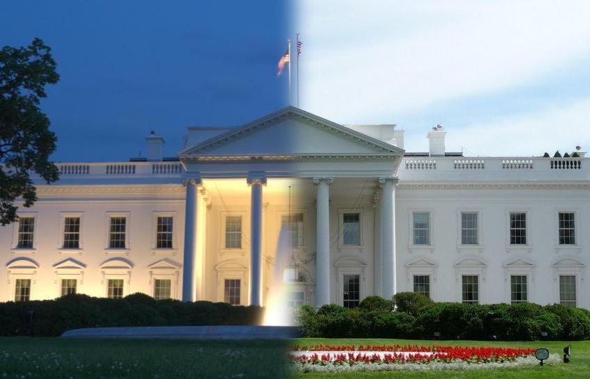
Day and night mosaic

I chose the white house images taken from day and night and compute the homography matrix and using pyramid blending method to compose both of them.

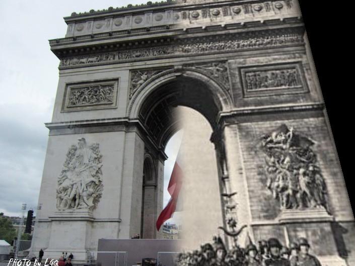
History mosaic

I chose the image of triumph gate in France. One is taken from modern time, the other is taken from World War 2. Same as previous pairs of images, I compute the homography matrix and using pyramid blending method to compose both of them.

Better Blending

Image pyramid blending has mainly four steps:(1) Build Laplacian pyramids \(LA\) and \(LB\) from image \(A\) and \(B\) (2)Build a Gaussian pyramid \(GR\) from selected region \(R\) (3) Form a combined pyramids \(LS\) from \(LA\) and \(LB\) using nodes of \(GR\) as weights: \(LS(i,j)=GR(i,j)*LA(i,j)+(1-GR(i,j))*LB(i,j)\)(4) Collapse the \(LS\) pyramid to get the final blended image.

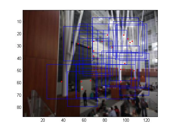
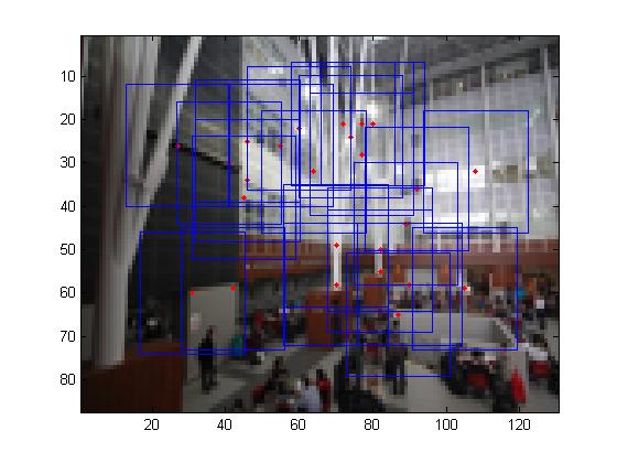
Multi-scale processing for corner detection and feature description

To produce multi-scale harris corners, the images was simply downsampled with a raito of 2. It should be noted that all all scales, the feature descriptors were taken from a 40*40 window before sampled to a 8*8 feature descriptor.

Rotation Invariant Descriptors

To make the descriptors invariant to image rotation, I assign a consistent orientation to each keypoint based on local image properties. The keypoint descriptor can be represented relative to this orientation and therefore achieve invariance to image rotation. The orientation is computed using the following equation:

\[\theta(x,y)=tan^-1((I(x,y+1)-I(x,y-1))/(L(x+1,y)-L(x-1,y)))\]

Panorama Recognition

For panorama recognition for input unordered image set, I do it using following steps:

1 Extract feature descriptor for all the images

2 Find nearest neighbor for each feature

3 For each image:1 Select m candidate matching images(with the maximum number of feature matches to this image) 2 Find geometrically consistent feature matches using the RANSAC to solve for the homography between pairs of images

4 Do the image stitching for each matched pairs of images